Introduction to value-based deep reinforcement learning

Brief of previous chapters

• chapter 2: learned to represent problems in a way reinforcement learning agents can solve using Markov decision process (MDP).
• chapter 3: developed algorithms that solve these MDPs.
• chapter 4: learned about algorithms that solve one-step MDPs, without having access to these MDPs.
• chapter 5: explore agents that learn to evaluate policies. Agent didn’t find optimal policies but were able to evaluate policies and estimate value function accurately.
• chapter 6: studied agents that find optimal policies on sequential decision-making problems under uncertainty.
• chapter 7: learned about agents that are even better at finding optimal policies by getting the most out of their experiences.

The algorithms mentioned earlier can be referred as tabular reinforcement learning.

The kind of feedback deep reinforcement learning agents use

In deep reinforcement learning, we build agents that are capable of learning from feedback that’s simultaneously evaluative, sequential, and sampled.

	Sequential (as opposed to one-shot)	Evaluative (as opposed to supervised)	Sampled (as opposed to exhaustive)
Supervised learning	✗	✗	✓
Planning (Chapter 3)	✓	✗	✗
Bandits (Chapter 4)	✗	✓	✗
Tabular reinforcement learning (Chapters 5, 6, 7)	✓	✓	✗
Deep reinforcement learning (Chapters 8, 9, 10, 11, 12)	✓	✓	✓

Deep reinforcement learning agents deal with sequential feedback

Deep reinforcement learning agents have to deal with sequential feedback. One of the main challenges of sequential feedback is that your agents can receive delayed information.

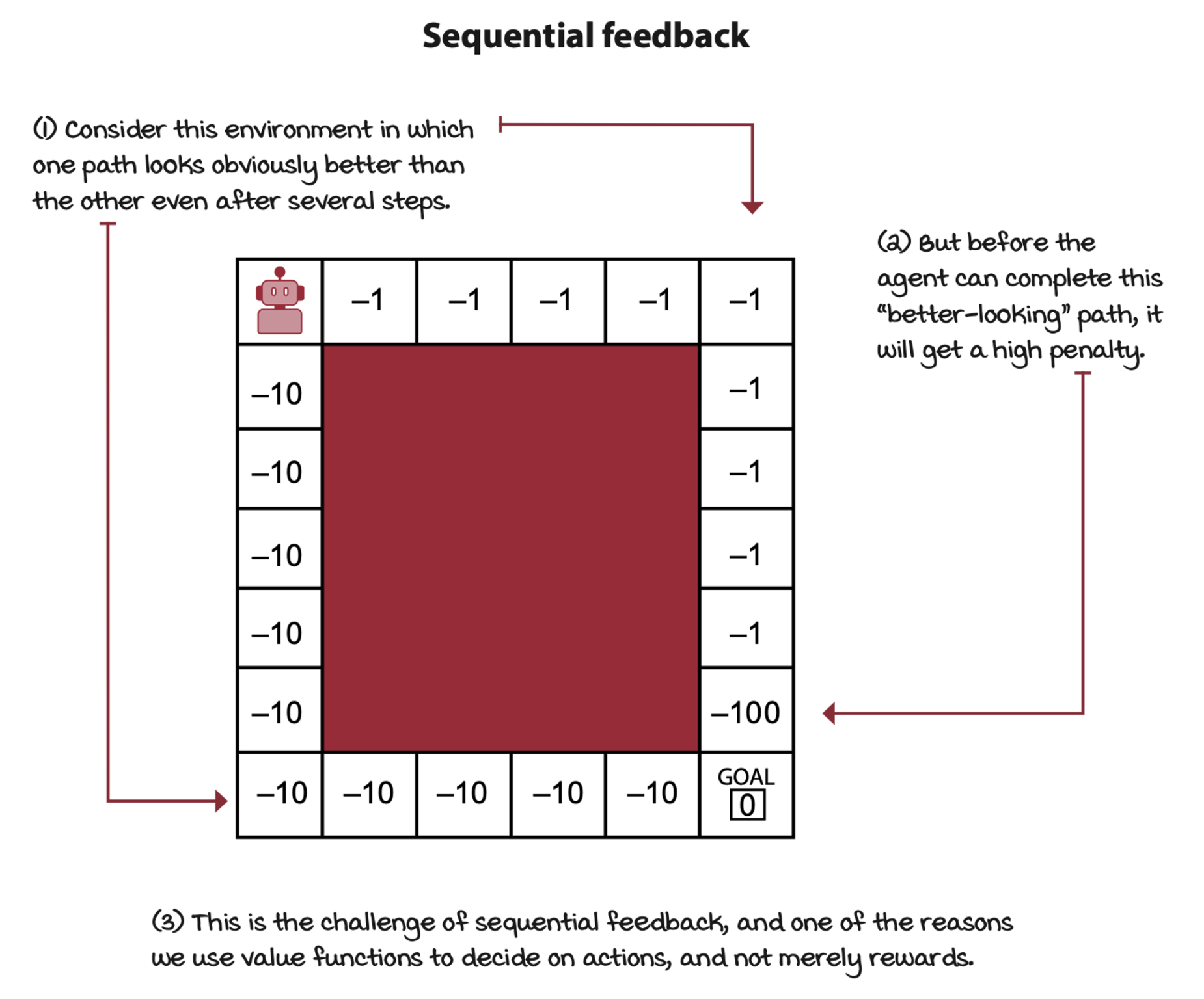
The opposite of delayed feedback is immediate feedback. In supervised learning or multi-armed bandits, decisions don’t have long-term consequences.

Deep reinforcement learning agents deal with evaluative feedback

The crux of evaluative feedback is that the goodness of the feedback is only relative, because the environment is uncertain. We don’t know the actual dynamics of the environment, we don’t have access to the trainsition function and reward signal.

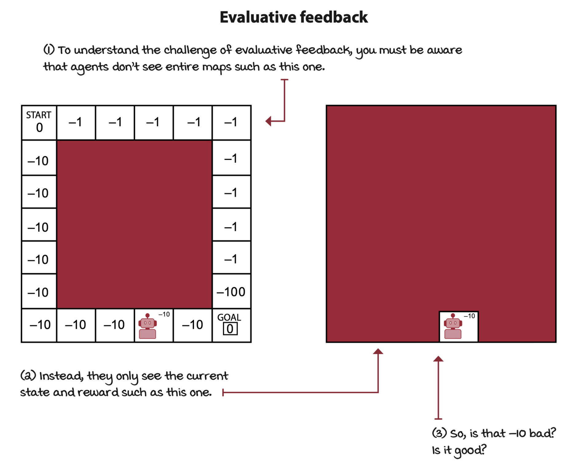
The opposite of evaluative feedback is supervised feedback.

Deep reinforcement learning agents deal with sampled feedback

In deep reinforcement learning, agents are unlikely to sample all possible feedback exhaustively. Agents need to generalize using the gathered feedback and come up with intelligent decisions based on that generalization.

The opposite of sampled feedback is exhausitive feedback. To exhaustively sample environments means agents have access to all possible samples.

Introduction to function approximation for reinforcement learning

Reinforcement learning problems can have high-dimensional state and action spaces

The main drawback of tabular reinforcement learning is that the use of a table to represent value functions is no longer practical in complex problems.

Reinforcement learning problems can have continuous state and action spaces

Environments can additionally have continuous variables, meaning that a variable can take on an infinite number of values.

Example: A cart-pole environment

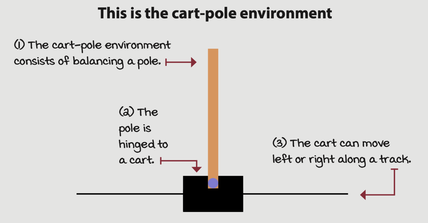
Its state space is comprised of four variables:

• The cart position on the track with a range from -2.4 to 2.4
• The cart velocity along the track with a range from -inf to inf
• The pole angle with a range of -40 degrees to 40 degrees
• The pole velocity at the tip with a range of -inf to inf

There are two available actions in every state:

• Action 0 applies a -1 force to the cart (push it left)
• Action 1 applies a +1 force to the cart (push it right)

You reach a terminal state if

• The pole angle is more than 12 degrees away from the vertical position
• The cart center is more than 2.4 units from the center of the track
• The episode count reaches 500 time steps

The reward function is

• +1 for every time step

NFQ: The first attempt at value-based deep reinforcement learning

The following algorithm is called neural fitted Q (NFQ) iteration.

First decision point: Selecting a value function to approximate

To begin with, we have to choose a value function to approximate.

• The state-value function \(v(s)\)
• The action-value function \(q(s, a)\)
• The action-advantage function \(a(s, a)\)

For now, let’s settle on estimating the action-value function \(q(s, a)\). We refer to the approximate action-value function estimate as \(Q(s, a; \theta)\), which mean the \(Q\) estimates are parameterized by \(\theta\), the weights of a neural network, a state \(s\) and an action \(a\).

Second decision point: Selecting a neural network architecture

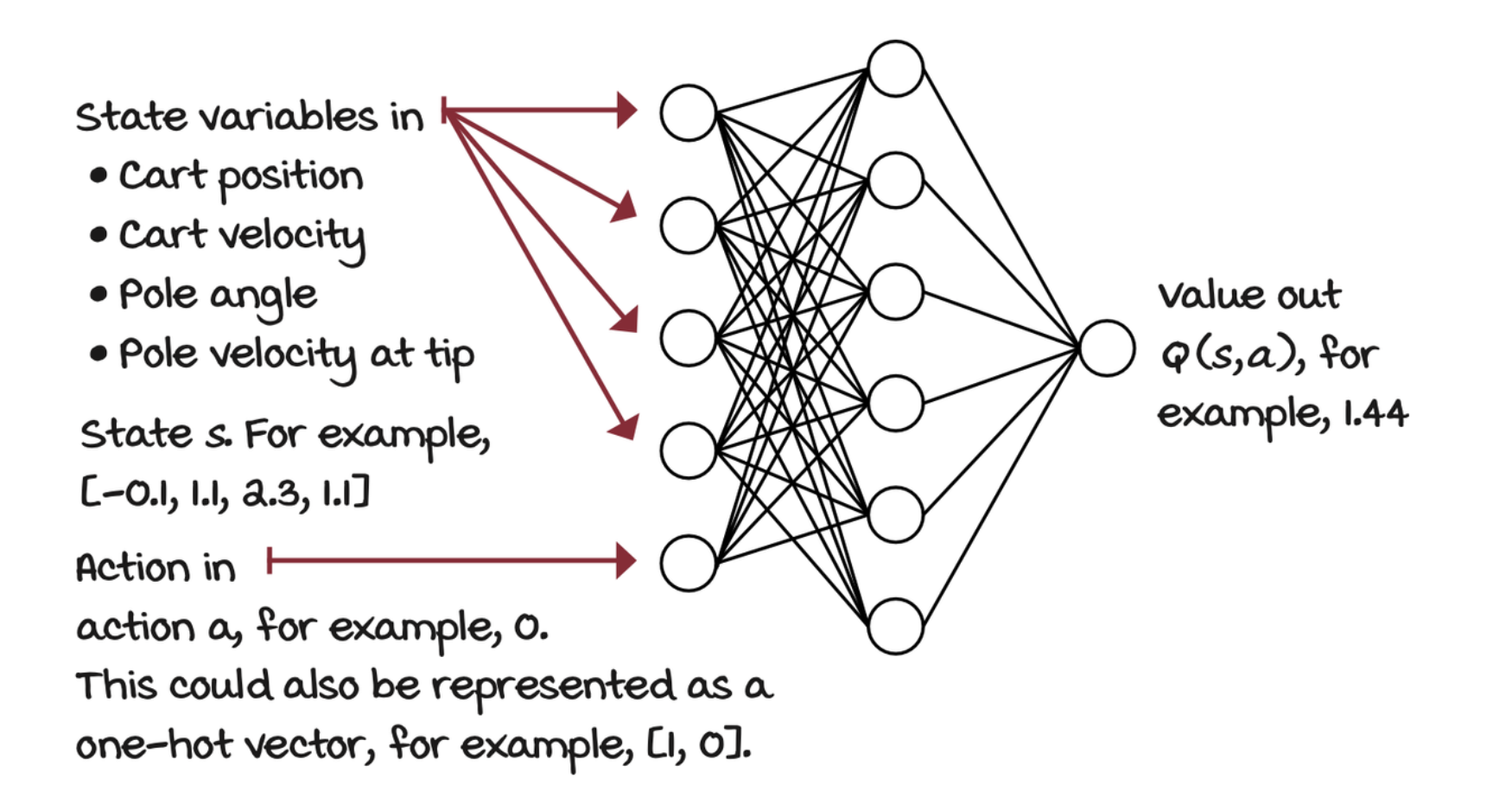
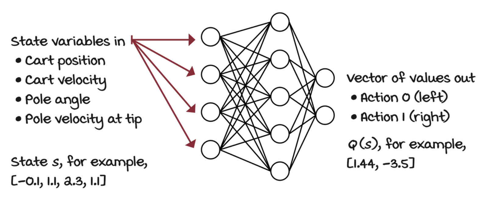
When we implemented the Q-learning agent, you noticed how the matrix holding the action-value function was indexed by state and action pairs. A straightforward neural network architecture is to input the state, and the action to evaluate. The output would then be one node representing the Q-value for that state action pair. But, a more efficient architecture consists of only inputting the state to the neural network and outputting the Q-values for all the actions in that state.

state-action-in-value-out-architecture

state-in-values-out-architecture

Third decision point: Selecting what to optimize

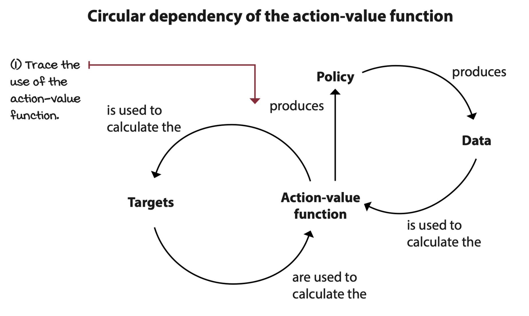
In the NFQ implementation, we start with a randomly initialized action-value function. Then we evaluate the policy by sampling actions from it. Then improve it with an exploration strategy such as epsilon-greedy. Finally, keep iterating until we reach the desired performance.

💡 Since we don’t have access to the optimal action-value function, and we don’t even have an optimal policy to sample from, we mush alternate between evaluating a policy (by sampling actions from it), and improving it (using an exploration strategy, such as epsilon-greedy).

Fourth decision point: Selecting the targets for policy evaluation

There are different targets we can use for estimating the action-value function of a policy \(\pi\). Such as MC target, TD target, the n-step target, or the lambda target.

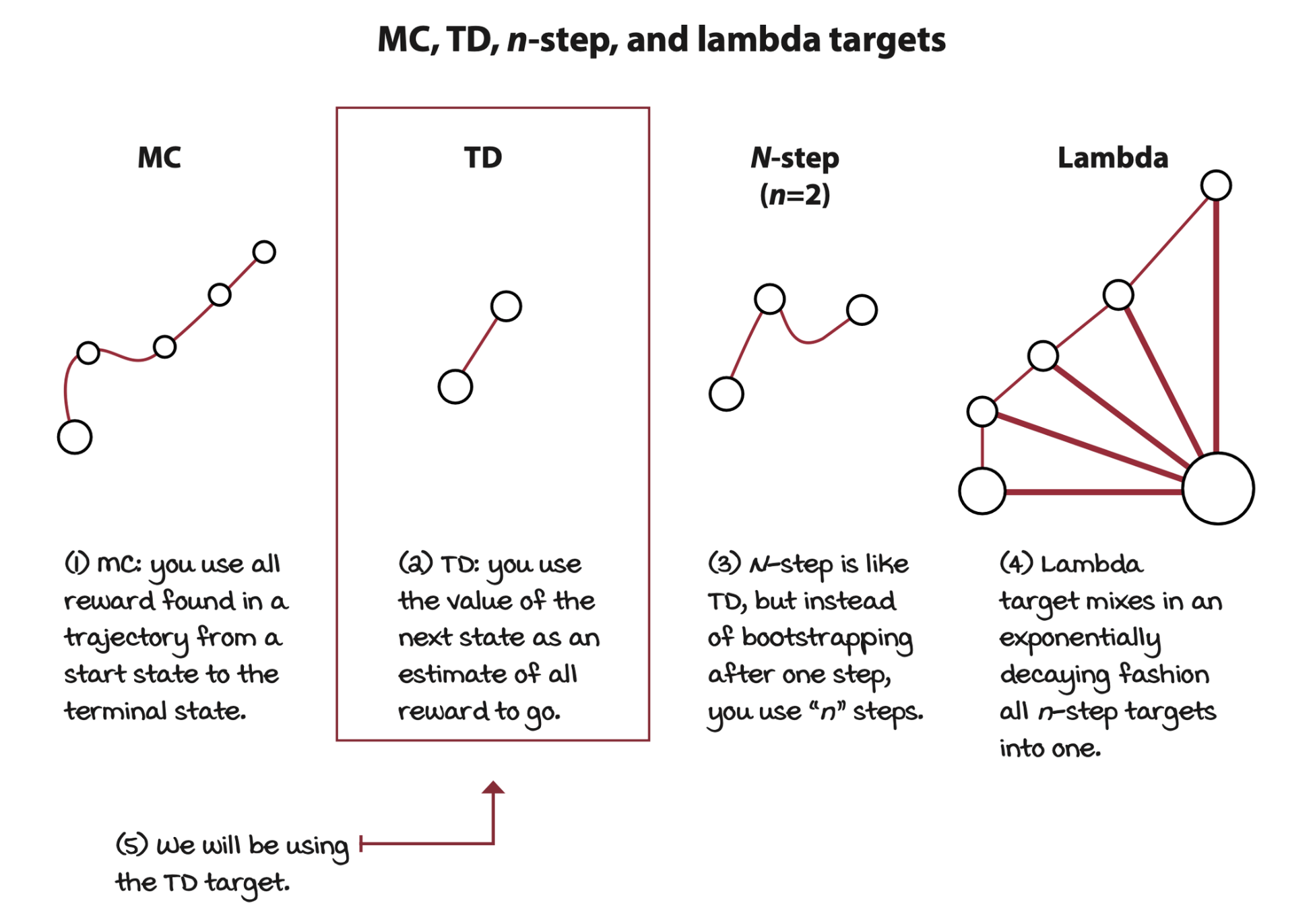
TD targets can be on-policy, which is called the SARSA target, or off-policy, which is called the Q-learning target.

\[ \begin{align*} y_i^\text{SARSA} &= R_{t+1} + \gamma Q(S_{t+1}, A_{t+1}; \theta_i) \\ y_i^\text{Q-learning} &= R_{t+1} + \gamma \max_a Q(S_{t+1}, a; \theta_i) \\ \end{align*} \]

The loss between a target and an estimate is

\[ L_i(\theta_i) = \Bbb E_{s, a, r, s'}[(r + \gamma \max_{a'} Q(s', a'; \theta_i) - Q(s, a; \theta_i))^2] \]

where \(\Bbb E_{s, a, r, s'}\) is the expectation of the experience tuple. \(r + \gamma \max_{a'} Q(s', a'; \theta_i)\) is a more general form of the Q-learning target. The differentiate the equation.

\[ \nabla_{\theta_i} L_i(\theta_i) = \Bbb E_{s, a, r, s'}[(r + \gamma \max_{a'} Q(s', a'; \theta_i) - Q(s, a; \theta_i)) \color{blue} \nabla_{\theta_i} Q(s, a; \theta_i) \color{black}] \]

Notice that the gradient must only go through the predicted value.

Fifth decision point: Selecting an exploration strategy

One interesting fact of off-policy learning algorithms is that the policy generating behavior can be virtually anything. That is, it can be anything as long as it has broad support, which means it must ensure enough exploration of all state-action pairs.

Sixth decision point: Selecting a loss function

Mean squared error (L2 loss) is a common loss function.

Seventh decision point: Selecting an optimization method

Gradient descent is a stable optimization method given a couple of assumptions: data must be independent and identically distributed (IID), and targets must be stationary. In reinforcement learning, however, we cannot ensure any of these assumptions hold, so choosing a robust optimization method to minimize the loss function can often make the difference between convergence and divergence.

The full algorithm

Selections we made

• Approximate the action-value function \(Q(s, a; \theta)\)
• Use a state-in-values-out architecture (nodes: 4, 512, 128, 2)
• Optimize the action-value function to approximate the optimal action-value function \(q^*(s, a)\)
• Use off-policy TD targets \((r + \gamma * \max_a' Q(s', a'; \theta))\) to evaluate policies
• Use an epsilon-greedy (\(\epsilon = 0.5\)) strategy to improve policies
• Use MSE for loss function
• Use RMSprop as the optimizer with a learning rate of 0.0005

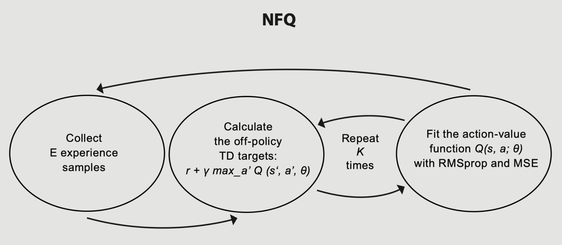
NFQ has three main steps:

1. Collect experiences tupes \((s, a, r, s', d)\)
2. Calculate the off-policy TD targets \((r + \gamma * \max_{a'} Q(s', a'; \theta))\)
3. Fit the action-value function \(Q(s, a;\theta)\) using MSE and RMSprop

Repeats step 2 and 3 \(K ( = 40)\) times before going back to step 1.