Curiosity-driven exploration

The games that DQN was successful at all gave relatively frequent rewards during game play and did not require significant long-term planning. But some other games, let’s say give a reward after the player finds a key in the room. But it is extremely unlikely that the agent will find the key and get a reward with this random exploration policy.

This problem is called the sparse reward problem. If the agent doesn’t observe enough reward signals to reinforce its actions, it can’t learn.

Tackling sparse rewards with predictive coding

Curiosity can be thought of as a kind of desire to reduce the uncertainty in your environment. One of the first attempts to imbue reinforcement learning agents with a sense of curiosity involved using a prediction error mechanism. The idea was that in addition to trying to maximize extrinsic rewards, the agent would also try to predict the next state of the environment given its action, and it would try to reduce its prediction error.

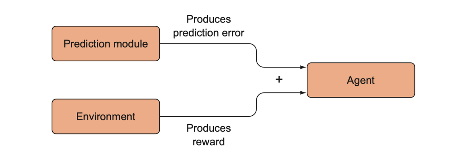
The idea is to sum the prediction error (which will be called intrinsic reward) with the extrinsic reward and use that total as the new reward signal for the environment.

💡 If you train these agents in an environment that has a constant source of randomness, such as TV screen playing random noise, the agent will have a constantly high prediction error and will be unable to reduce it.

Inverse dynamics prediction

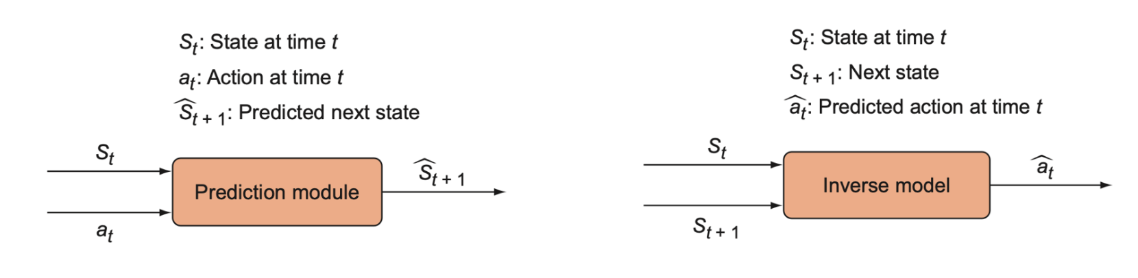
The prediction error module is implemented as a function: \(f: (S_t, a_t) \to \hat{S}_{t+1}\), that takes a state and the action taken and returns the predicted next state. It is predicting the future state of the environment, so we call it the forward-prediction model.

We want to only predict aspects of the state that actually matter, not parts that are trivial or noise. The way to build in the “doesn’t matter” constraint to the prediction model is to add another model called an inverse model, \(g: (S_t, S_{t+1}) \to \hat{a}_t\). This is a function that takes a state and the next state, and then returns a prediction for which action was taken that led to the transition from \(s_t\) to \(s_{t+1}\).

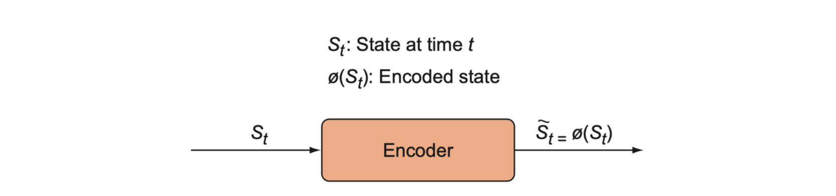
There is another model that is tightly coupled to the inverse model called the encoder model, denoted \(\phi\). The encoder function, \(\phi: S_t \to \tilde{S}_t\), takes a state and returns an encoded state \(\tilde{S}_t\) such that the dimensionality of \(\tilde{S}_t\) is significantly lower than the raw state \(S_t\).

The encoder model is trained via the inverse model because we actually use the encoded states as inputs to the forward and inverse models \(f\) and \(g\) rather than the raw states. That is, the forward model becomes a function, \(f: \phi(S_t) \times a_t \to \hat{\phi}(S_{t+1})\), where \(\hat{\phi}(S_{t+1})\) refers to a prediction of the encoded state, and the inverse model becomes \(g: \phi(S_t) \times \hat{\phi}(S_{t+1}) \to \hat{a}_t\).

The encoder model isn’t trained directly —— it is not an auto-encoder. It is only trained through the inverse model.

The curiosity module.

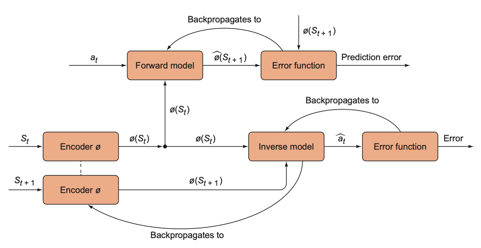
1. Encode states \(S_t\) and \(S_{t+1}\) into low-dimensional vectors, \(\phi(S_t)\) and \(\phi(S_{t+1})\).
2. The encoded states are passed to the forward and inverse models.
3. The inverse model backpropagates to the encoded model.
4. The forward model is trained by backpropagating from its own error function, but it does not backpropagate through to the encoder.

Setting up Super Mario Bros

The forward, inverse, and encoder models form the intrinsic curiosity module (ICM), which will be implemented below. The ICM generates a new intrinsic reward signal based on information from the environment, so it is independent of how the agent model is implemented. To keep everything simple, we use a Q-learning model.

Install Super Mario Bros by pip.

pip install gym-super-mario-bros

After installing, it can be used as

from nes_py.wrappers import JoypadSpace
import gym_super_mario_bros
from gym_super_mario_bros.actions import SIMPLE_MOVEMENT, COMPLEX_MOVEMENT

env = gym_super_mario_bros.make(
    'SuperMarioBros-v0',
    apply_api_compatibility=True,
    render_mode='human')
env = JoypadSpace(env, COMPLEX_MOVEMENT)

render_mode specifies how the game is rendered. In most of training processes below, the render_mode is rgb_array, which returns an array of a frame in the game, whose shape is (x, y, 3)

Since gym now becomes gymnasium, all the APIs have breaking changes, apply_api_compatibility should be set to True.

Preprocessing and the Q-network

The raw state is an RGB video frame with dimensions (240, 256, 3), which is unnecessarily high-dimensional and would be computationally costly for no advantage. We will convert these RGB states into grayscale and resize them to 42x42 to allow our model to train much faster.

import matplotlib.pyplot as plt
from skimage.transform import resize
import numpy as np

def downscale_obs(obs, new_size=(42, 42), to_gray=True):
    if to_gray:
        return resize(obs, new_size, anti_aliasing=True).max(axis=2)
    else:
        return resize(obs, new_size, anti_aliasing=True)

Then we will use the last three frames as a single state. This gives our model access to velocity information.

Each state given to the agent is a concatenation of the three most recent (grayscale) frames in the game. This is necessary so that the model can have access to not just the position of objects, but also their direction of movement.

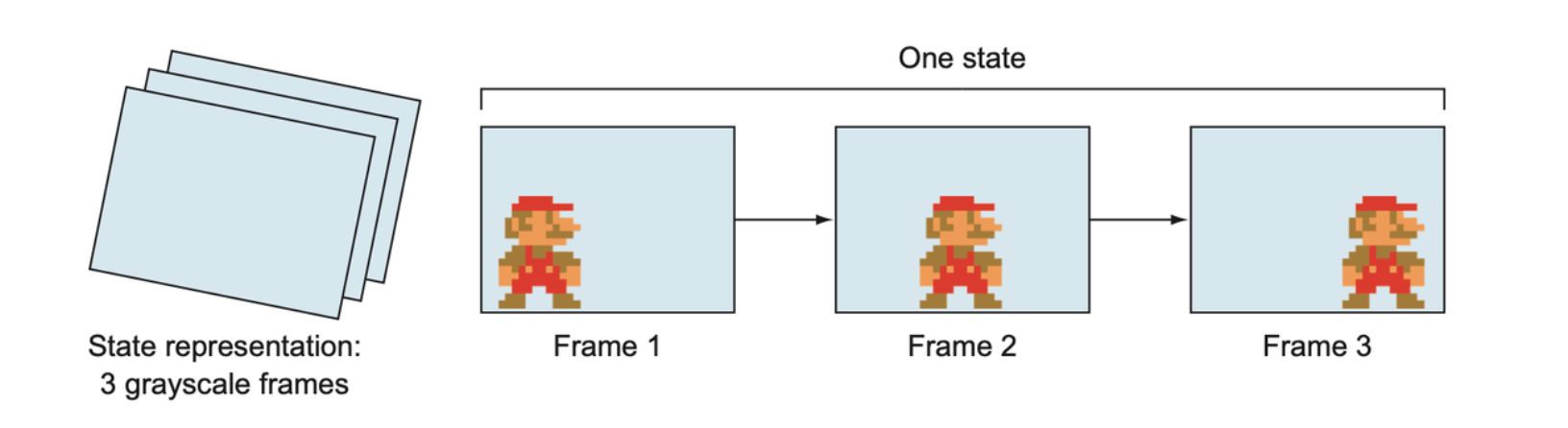
Each state given to the agent is a concatenation of the three most recent (grayscale) frames in the game. This is necessary so that the model can have access to not just the position of objects, but also their direction of movement.

We need three functions to handle the states:

• prepare_state(state): Downscale state and converts to grayscale, converts to a pytorch tensor and adds a batch dimension.
• prepare_multi_state(state1, state2): Given an existing 3-frame state1 and a new single frame2, adds the latest frame to the queue.
• prepare_initial_state(state, N=3): Creates a state with three copies of the same frame and adds a batch dimension.

Setting up the Q-network and policy function

DQN is used for our agent here. It is consisted with four layers of convolution networks. The activation function used here is ELU. DQN needs a policy function, which selects action from the Q values return by DQN.

Policy function

We will use a policy that begins with a softmax policy to encourage exploration, and after a fixed number of game steps we will switch to an epsilon-greedy strategy.

def policy(qvalues, eps=None):
    if eps is not None:
        if torch.rand(1) < eps:
            return torch.randint(low=0, high=11, size=(1,))
        else:
            return torch.argmax(qvalues)
    else:
      return torch.multinomial(F.softmax(F.normalize(qvalues)),
                               num_samples=1)

If eps is not provided, we sample from the softmax of Q values.

Experience replay

An experience replay class contains a list of experiences, each of which is a tuple of \((S_t, a_t, r_t, S_{t+1})\).

from random import shuffle
import torch
from torch import nn
from torch import optim
import torch.nn.functional as F

class ExperienceReplay:
    def __init__(self, N=500, batch_size=100):
        self.N = N
        self.batch_size = batch_size
        self.memory = []
        self.counter = 0

    def add_memory(self, state1, action, reward, state2):
        self.counter += 1
        if self.counter % 500 == 0:
            self.shuffle_memory()

        # if the memory is not full, adds to the list
        # otherwise replaces a random memory with the new one
        if len(self.memory) < self.N:
            self.memory.append((state1, action, reward, state2))
        else:
            rand_index = np.random.randint(0, self.N - 1)
            self.memory[rand_index] = (state1, action, reward, state2)

    def shuffle_memory(self):
        shuffle(self.memory)

    def get_batch(self):
        if len(self.memory) < self.batch_size:
            batch_size = len(self.memory)
        else:
            batch_size = self.batch_size
        
        if len(self.memory) < 1:
            print('Error: No data in memory.')
            return None

        indexes = np.random.choice(
                  np.arange(len(self.memory)), batch_size, replace=False)
        batch = [self.memory[i] for i in indexes]
        state1_batch = torch.stack([x[0].squeeze(dim=0) for x in batch], dim=0)
        action_batch = torch.Tensor([x[1] for x in batch]).long()
        reward_batch = torch.Tensor([x[2] for x in batch])
        state2_batch = torch.stack([x[3].squeeze(dim=0) for x in batch], dim=0)
        return state1_batch, action_batch, reward_batch, state2_batch

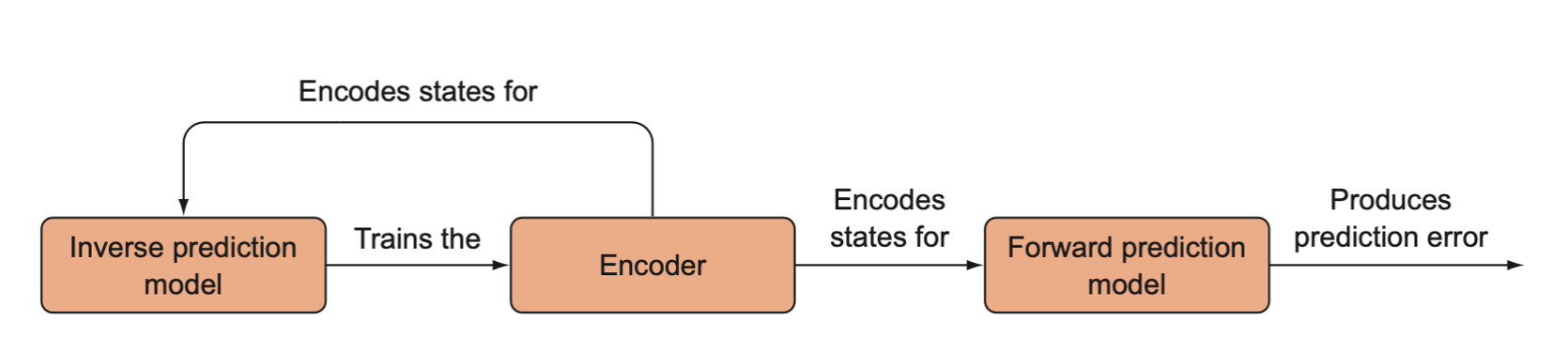
Intrinsic curiosity module

A high-level overview of the intrinsic curiosity module (ICM). The ICM has three components that are each separate neural networks. The encoder model encodes states into a low-dimensional vector, and it is trained indirectly through the inverse model, which tries to predict the action that was taken given two consecutive states. The forward model predicts the next encoded state, and its error is the prediction error that is used as the intrinsic reward.

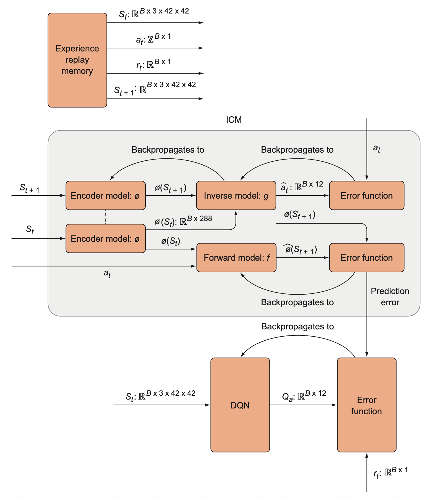
Below shows the type and dimensionality of the inputs and outputs of each component of the ICM.

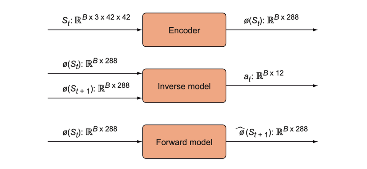
The DQN and the ICM contribute to a single overall loss function that is given to the optimizer to minimize with respect to the DQN and ICM parameters. The DQN’s Q value predictions are compared to the observed rewards. The observed rewards, however, are summed together with the ICM’s prediction error to get a new reward value.

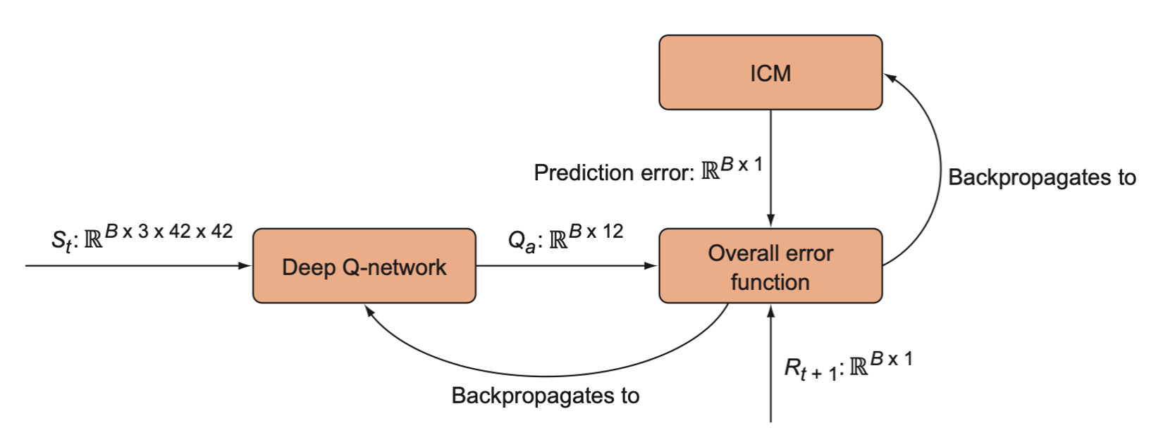
A complete view of the overall algorithm, including the ICM. First we generate \(B\) samples from the experience replay memory and use these for the ICM and DQN. We run the ICM forward to generate a prediction error, which is then provided to the DQN’s error function. The DQN learns to predict action values that reflect not only extrinsic (environment provided) rewards but also an intrinsic (prediction error-based) reward.

• The forward model is a simple two-layer neural network with linear layers.
• The inverse model is also a simple two-layer neural network with linear layers.
• The encoder is a neural network composed of four convolutional layers (with an identical architecture to the DQN)

The overall loss function defined by all four models is

\[ \text{minimize} [\lambda \cdot Q_\text{loss} + (1 - \beta)F_\text{loss} + \beta \cdot G_\text{loss}] \]

ICM

def ICM(state1, action, state2, forward_scale=1., inverse_scale=1e4):
    # encodes state1 and state2
    state1_hat = encoder(state1)
    state2_hat = encoder(state2)

    # runs forward model to get state2 prediction
    state2_hat_pred = forward_model(state1_hat.detach(), action.detach())
    # calculates forward loss
    forward_pred_err = forward_scale * \
        forward_loss(state2_hat_pred, state2_hat.detach()).sum(dim=1).unsqueeze(dim=1)
    # runs inverse model to get action prediction
    pred_action = inverse_model(state1_hat, state2_hat)
    # calculates inverse loss
    inverse_pred_err = inverse_scale * \
        inverse_loss(pred_action, action.detach().flatten()).unsqueeze(dim=1)
  
    return forward_pred_err, inverse_pred_err

Mini-batch train

def minibatch_train(use_extrinsic=True):
    state1_batch, action_batch, reward_batch, state2_batch = replay.get_batch()
    action_batch = action_batch.view(action_batch.shape[0], 1)
    reward_batch = reward_batch.view(reward_batch.shape[0], 1)
    
    # gets losses of forward model and inverse model
    forward_pred_err, inverse_pred_err = ICM(state1_batch, action_batch, state2_batch)
    i_reward = (1. / params['eta']) * forward_pred_err
    reward = i_reward.detach()

    if use_extrinsic:
        reward += reward_batch

    # calculates Q values for the next state
    qvals = Qmodel(state2_batch)
    reward += params['gamma'] * torch.max(qvals)
    reward_pred = Qmodel(state1_batch)
    reward_target = reward_pred.clone()

    # since the action_batch is a tensor of integers of action indices,
    # we convert this to a tensor of one-hot encoded vectors.
    indices = torch.stack((torch.arange(action_batch.shape[0]), action_batch.squeeze()), dim=0)
    indices = indices.tolist()
    reward_target[indices] = reward.squeeze()
    q_loss = 1e5 * qloss(F.normalize(reward_pred), F.normalize(reward_target.detach()))
    return forward_pred_err, inverse_pred_err, q_loss

Main training loop

The final training process is defined as follows:

from IPython.display import clear_output

env = get_env('rgb_array')

epochs = 3500
env.reset()

state1 = prepare_initial_state(env.render())
eps = 0.15 # epsilon in policy method
losses = []
episode_length = 0
switch_to_eps_greedy = 1000 # use epsilon greedy after 1000 episodes
state_deque = deque(maxlen=params['frames_per_state'])
e_reward = 0.
# last_x_pos = env.env.env._x_position
last_x_pos = 0
ep_lengths = []
use_extrinsic = False

for i in range(epochs):
    opt.zero_grad()
    episode_length += 1
    # runs DQN to get Q values
    q_val_pred = Qmodel(state1)
    if i > switch_to_eps_greedy:
        action = int(policy(q_val_pred, eps))
    else:
        action = int(policy(q_val_pred))
      
    # repeats actions for accelerating learning process
    for j in range(params['action_repeats']):
        state2, e_reward_, done, truncated, info = env.step(action)
        last_x_pos = info['x_pos']
        if done:
            state1 = reset_env()
            break
        e_reward += e_reward_
        state_deque.append(prepare_state(state2))
  
    state2 = torch.stack(list(state_deque), dim=1)
    replay.add_memory(state1, action, e_reward, state2)
    e_reward = 0
  
    if episode_length > params['max_episode_len']:
        if (info['x_pos'] - last_x_pos) < params['min_progress']:
            done = True
        else:
            last_x_pos = info['x_pos']
    if done:
        ep_lengths.append(info['x_pos'])
        state1 = reset_env()
        # last_x_pos = env.env.env._x_position
        last_x_pos = info['x_pos']
        episode_length = 0
    else:
        state1 = state2
  
    if len(replay.memory) < params['batch_size']:
        continue
  
    forward_pred_err, inverse_pred_err, q_loss = minibatch_train(use_extrinsic=False)
    loss = loss_fun(q_loss, forward_pred_err, inverse_pred_err)
    loss_list = (q_loss.mean(), forward_pred_err.flatten().mean(), inverse_pred_err.flatten().mean())
    losses.append(loss_list)
    loss.backward()
    opt.step()