Alternative optimization methods - Evolutionary algorithms

A different approach to reinforcement learning

With both DQN and policy gradient, we need to carefully tune several hyperparameters ranging from selecting the right optimizer function, mini-batch size, and learning rate so that the training would be stable and successful. Since the training of both DQN and policy gradient algorithms relies on stochastic gradient descent, there is no guarantee that these methods will successfully learn.

Moreover, in order to use gradient descent and back-propagation, we need a model that is differentiable.

Instead of creating one agent and improving it, we can instead learn from natural selection. We could spawn multiple different agents with different parameters, observe which ones did the best, and “breed” the best agents such that descendants could inherit their parent’s desirable traits.

Evolutionary algorithms are different from gradient descent-based optimization techniques. With evolutionary strategies, we generate agents and pass the most favorable weights down to the subsequent agents.

Reinforcement learning with evolution strategies

Evolution in theory

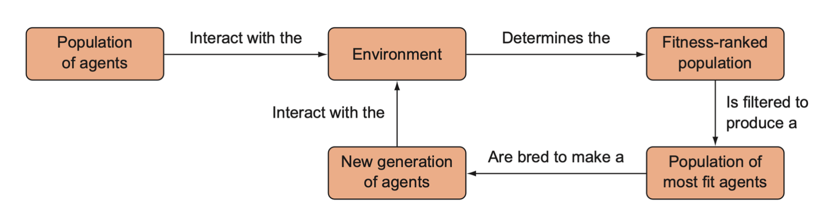
Natural selection selects for the “most fit” individuals from each generation. In biology this represents the individuals that had the greatest reproductive success, and hence passed on their genetic information to subsequent generations. The environment can be thought as determining an objective or fitness function that assigns individuals a fitness score based on their performance with that environment.

In evolutionary reinforcement learning, we are selecting for traits that give our agents the highest reward in a given environment, and by traits we mean model parameters or entire model structures. An RL agent’s fitness can be determined by the expected reward it would receive if it were to perform in the environment.

The objective in evolutionary reinforcement learning is exactly the same as in back-propagation and gradient descent-based training. The only difference is that we use this evolutionary process, which is often referred to as a genetic algorithm, to optimize the parameters of a model such as a neural network.

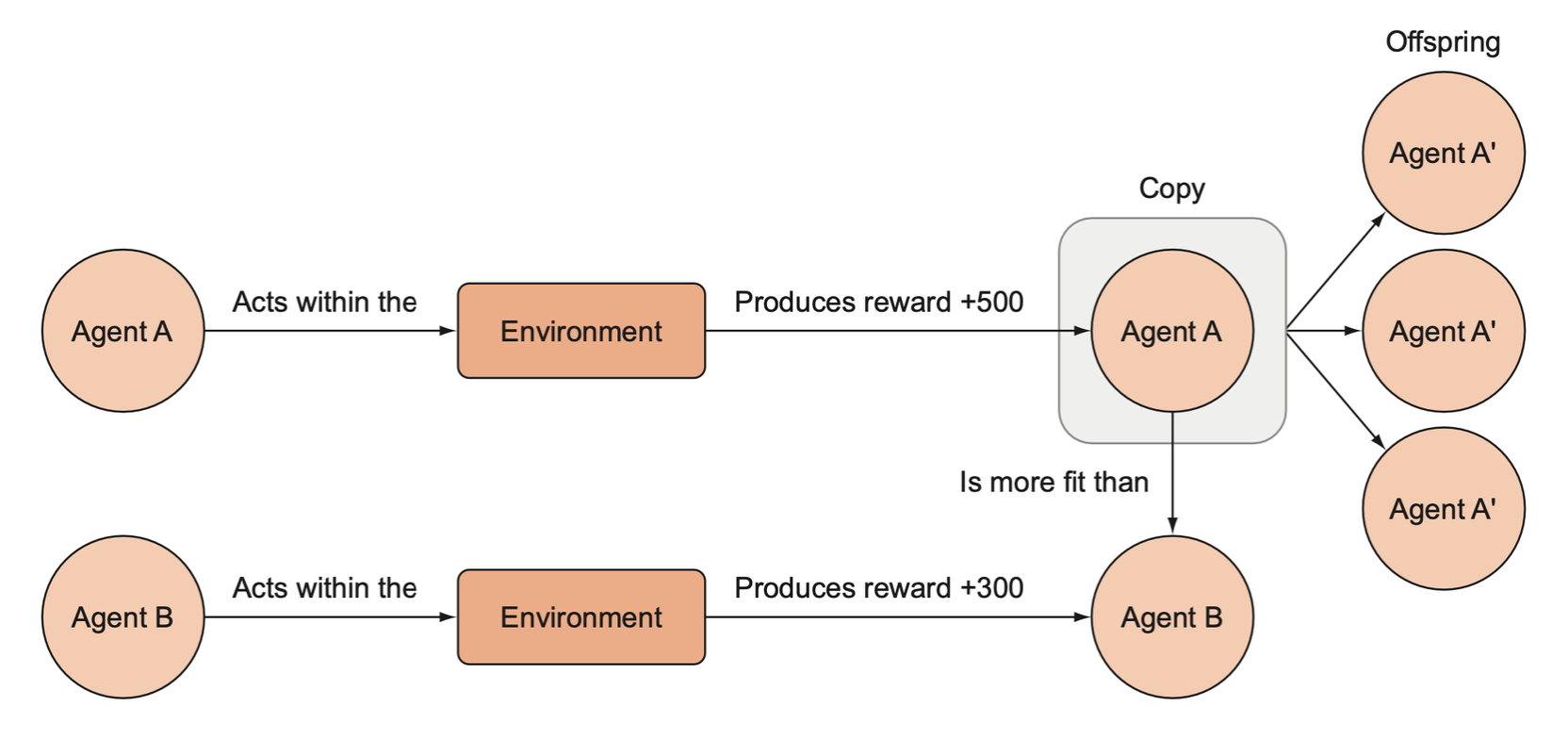
In an evolutionary algorithm approach to reinforcement learning, agents compete in an environment, and the agents that are more fit (those that generate more rewards) are preferentially copied to produce offspring. After many iterations of this process, only the most fit agents are left.

Training process

Train process is described as below:

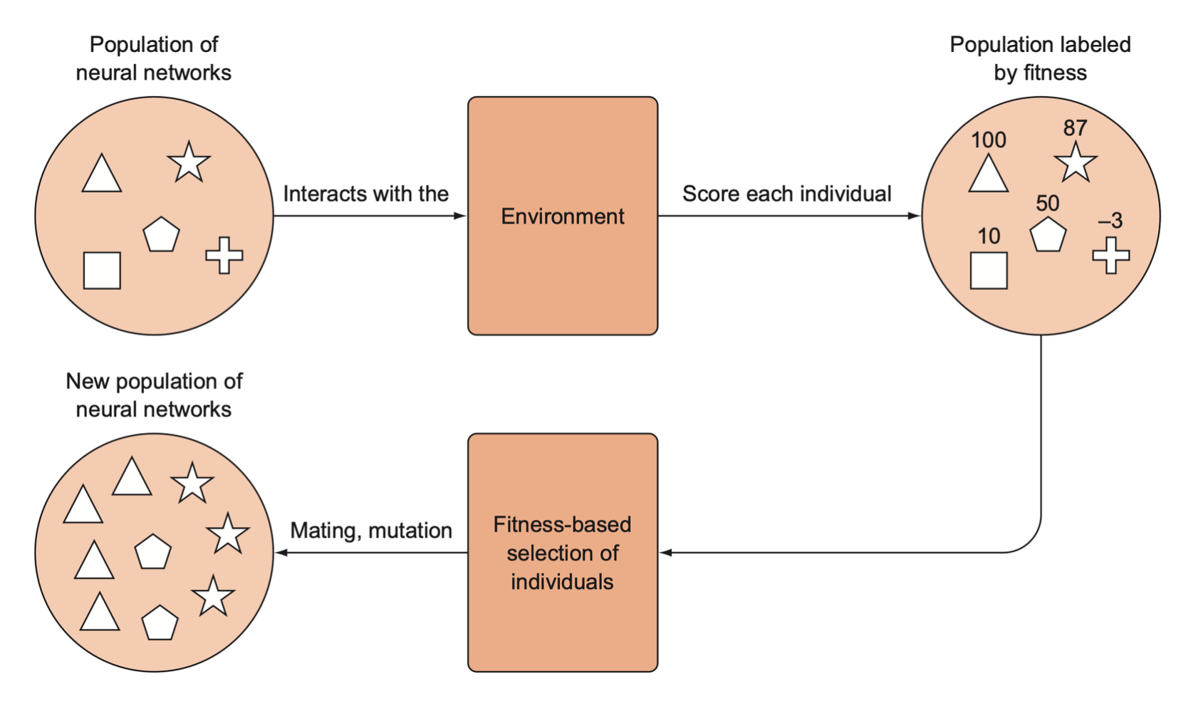
1. We generate an initial population of random parameter vectors. We refer to each parameter vector in the population as an individual.
2. We iterate through this population and assess the fitness of each individual by running the model in environment with that parameter vector and recording the rewards. Each individual is assigned a fitness score based on the rewards it earns.
3. We randomly sample a pair of individuals from the population, weighted according to their relative fitness score to create a “breeding population”.
4. The individuals in the breeding population will then “mate” to produce “offspring” that will form a new, full population. If the individuals are simply parameter vectors of real numbers, mating vector 1 with vector 2 involves taking a subset from vector 1 and combining it with a complementary subset of vector 2 to make a new offspring vector of the same dimensions.
5. With the new offspring solutions, we will iterate over our solutions and randomly mutate some of them to make sure we introduce new genetic diversity into every generation to prevent premature convergence on a local optimum. Mutation simply means adding a little random noise to the parameter vectors.
6. Repeat this process with the new population for \(N\) number of generations or until we reach convergence.

Pros and cons of evolutionary algorithms

There are circumstances where an evolutionary approach works better, such as with problems that would benefit more from exploration; other circumstances make it impractical, such as problems where it is expensive to gather data.

Evolutionary algorithms explore more

Both DQN and policy gradients followed a similar approach: collect experiences and nudge the agent to take actions that led to greater rewards. This tends to cause agents to abandon exploring new states if they prefer an action already.

The agents in the genetic algorithm, on the other hand, are not nudged in any direction.

Evolutionary algorithms are incredibly sample intensive

We have to make a lot of computation to calculate a bunch of random agents before we can actually evaluate them. We will say that evolutionary algorithms are less data-efficient than DQN or PG methods.

Being data-inefficient is a problem if collecting data is expensive, such as in robotics or with autonomous vehicles.

Simulators

Instead of using an expensive robot or building a car with the necessary sensors, we could instead use computer software to emulate the experiences the environment would provide. Not only are simulators significantly cheaper to train agents with, but agents are able to train much more quickly since they can interact with the simulated environment much faster than in real life.

Evolutionary algorithms as a scalable alternative

Producing a viable agent with evolutionary algorithms can sometimes be faster than gradient-based approaches because we do not have to compute the gradients via back-propagation. Another advantage of evolutionary algorithms is that they can be scaled incredibly well when parallelized.

Scaling evolutionary algorithms

Evolutionary algorithm is an umbrella term for a wide variety of algorithms that take inspiration from biological evolution and rely on interactively selecting slightly better solutions from a large population to optimize a solution.

There is another class of evolutionary algorithms confusingly termed evolutionary strategies (ES), which employ a less biologically accurate form of evolution.

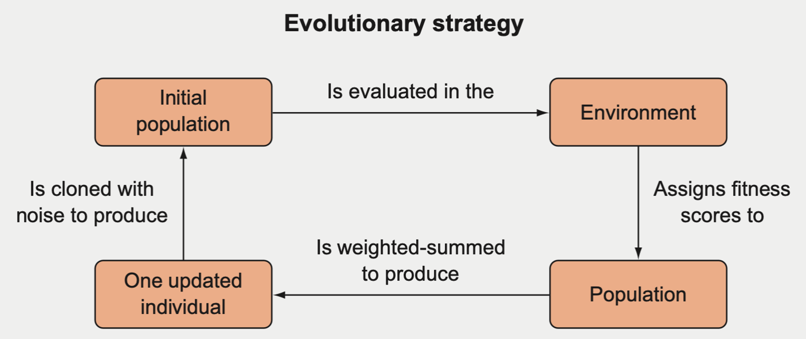
If we’re training a neural network with an ES algorithm

1. Start with a single parameter vector \(\theta_t\), sample a bunch of noise vectors of equal size (usually from a Gaussian distribution), such as \(e_i \sim N(\mu, \sigma)\).

2. Then create a population of parameter vectors that are mutated versions of \(\theta_t\) by taking \(\theta_i' = \theta + e_i\).

3. Test each of these mutated parameter vectors in the environment and assign them fitness scores based on their performance in the environment.

4. Get an updated parameter vector by taking a weighted sum of each of the mutated vectors, where the weights are proportional to their fitness scores.

   \[ \theta_{t+1} = \theta_t + \alpha \frac{1}{N_\sigma} \sum_i^N F_i \cdot e_i \]

   where the variables are defined as below:

   • \(\theta_{t+1}\): parameter vector
   • \(\alpha\): learning rate
   • \(N_\sigma\): population size
   • \(F_i\): fitness score
   • \(e_i\): noice vector

💡 This evolutionary strategy algorithm is significantly simpler than the genetic algorithm. We only perform mutation, and the recombination step does not involve swapping pieces from different parents but is just a simple weighted summation which is very easy to implement and computationally fast.

Parallel vs. serial processing

In the CartPole example, we determine the fitness of the agents one by one, which will generally be the longest-running task in an evolutionary algorithm.

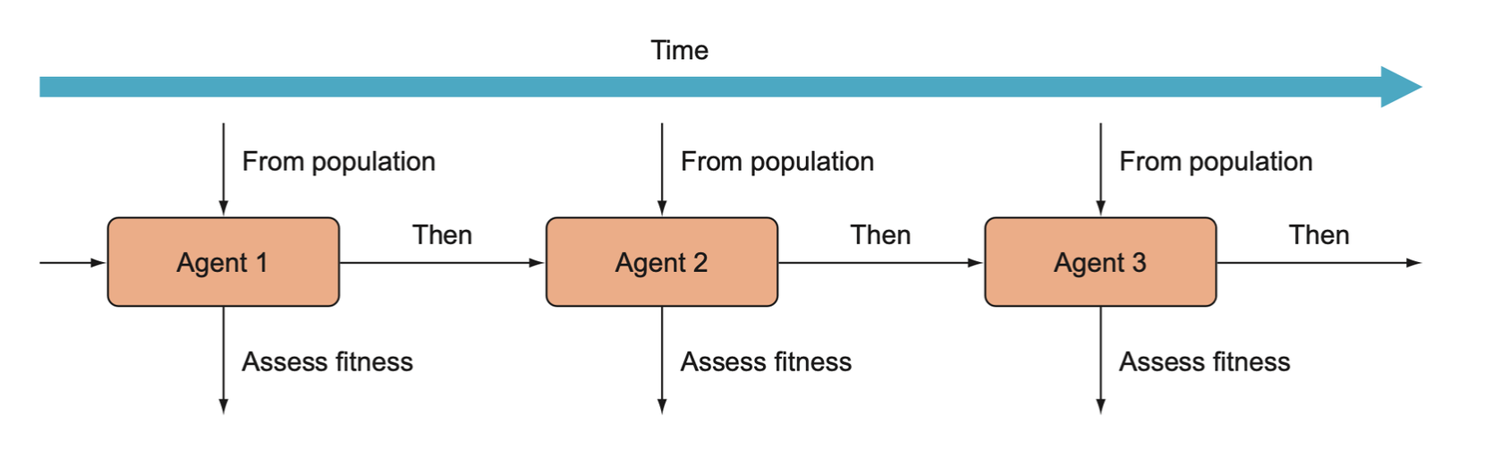
But we can determine the fitness simultaneously.

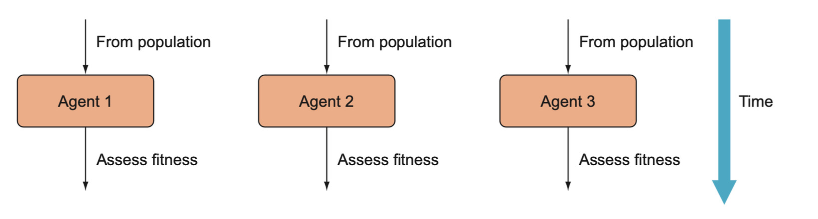
If we have multiple machines at our disposal, we can determine the fitness of each agent on its own machine in parallel with each other.

Scaling efficiency

Scaling efficiency is a term used to describe how a particular approach improves as more resources are thrown at it and can be calculated as follows:

\[ \text{Scaling Efficiency} = \frac{\text{Multiple of Performance Speed up after adding Resources}}{\text{Multiple of Resources Added}} \]

In the real world, processes never have a scaling efficiency of 1. Adding 10 more machines will only gives us a 9x speedup.

Ultimately we need to combine the results from assessing the fitness of each agent in parallel so that we can recombine and mutate them. Thus, we need to use true parallel processing followed by a period of sequential processing.

A general schematic for how distributed computing works. A master node assigns tasks to worker nodes; the worker nodes perform those tasks and then send their results back to the master node (not shown).

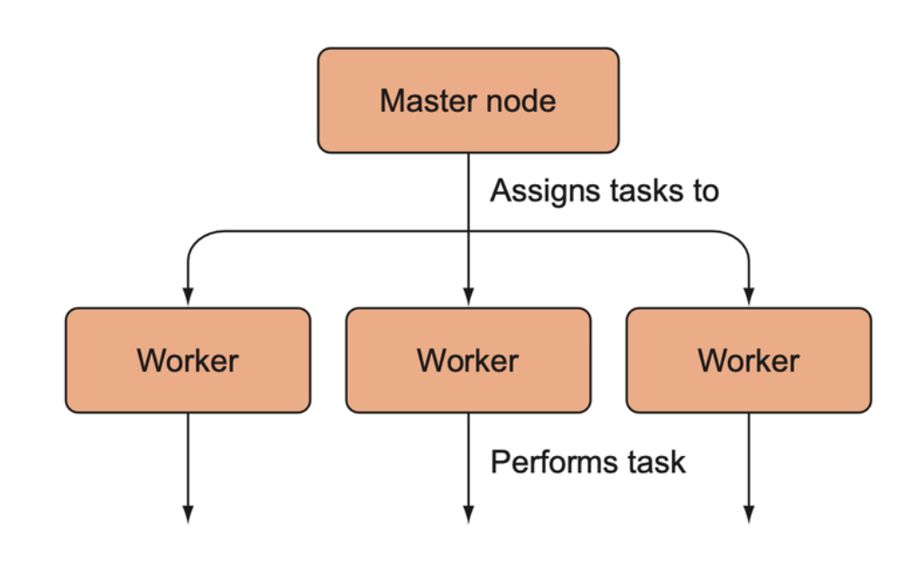
A general schematic for how distributed computing works. A master node assigns tasks to worker nodes; the worker nodes perform those tasks and then send their results back to the master node (not shown).

Communicating between nodes

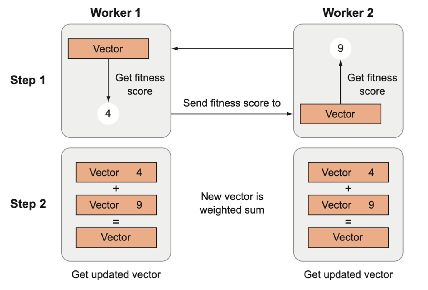
The architecture derived from OpenAI’s distributed ES paper. Each worker creates a child parameter vector from a parent by adding noise to the parent. Then it evaluates the child’s fitness and sends the fitness score to all other agents. Using shared random seeds, each agent can reconstruct the noise vectors used to create the other vectors from the other workers without each having to send an entire vector. Lastly, new parent vectors are created by performing a weighted sum of the child vectors, weighted according to their fitness scores.

💡 Seeing is important; it allows experiments involving random numbers to be reproduced by other researchers.

Scaling linearly

Scaling linearly means that for every machine added, we receive roughly the same performance boost as we did by adding the previous machine.

Figure recreated from the OpenAI “Evolutionary Strategies as a Scalable Alternative to Reinforcement Learning” paper. The figure demonstrates that as more computing resources were added, the time improvement remained constant.

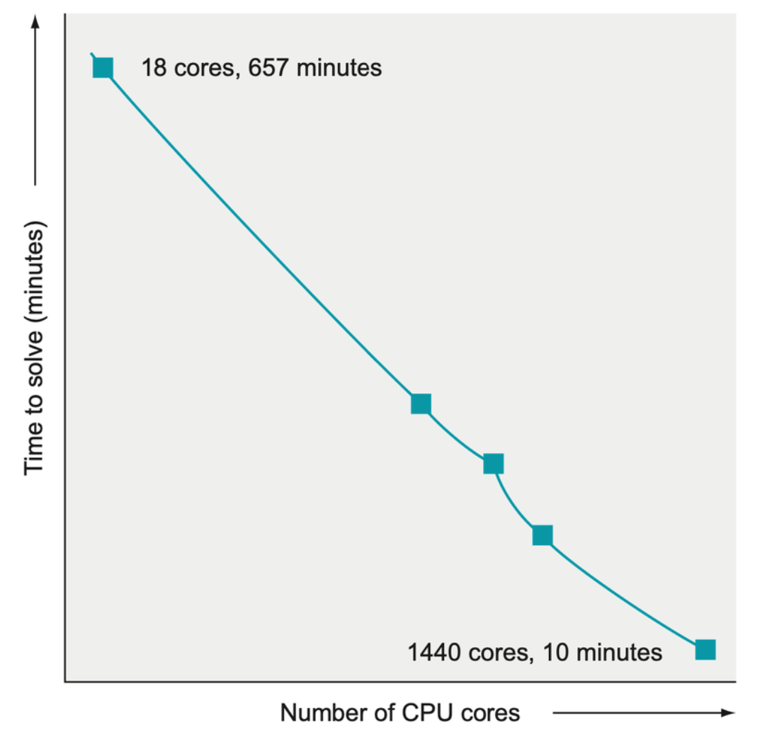
Figure recreated from the OpenAI “Evolutionary Strategies as a Scalable Alternative to Reinforcement Learning” paper. The figure demonstrates that as more computing resources were added, the time improvement remained constant.

Scaling gradient-based approaches

Gradient-based approaches can be trained on multiple machines as well. Currently, most distributed training of gradient-based approaches involves training the agent on each worker and then passing the gradients back to a central machine to be aggregated. All the gradients must be passed for each epoch or update cycle, which requires a lot of network bandwidth and strain on the central machine.

Summary

• Evolutionary algorithms provide us with more powerful tools for our toolkit. Based on biological evolution, we
  • Produce individuals
  • Select the best from the current generation
  • Shuffle the genes around
  • Mutate them to introduce some variation
  • Mate them to create new generations for the next population
• Evolutionary algorithms tend to be more data hungry and less data-efficient than gradient-based approaches; in some circumstances this may be fine, notably if you have a simulator.
• Evolutionary algorithms can optimize over non-differentiable or even discrete functions, which gradient-based methods cannot do.
• Evolutionary strategies (ES) are a subclass of evolutionary algorithms that do not involve biological-like mating and recombination, but instead use copying with noise and weighted sums to create new individuals from a population.