Distributional DQN - Getting the full story

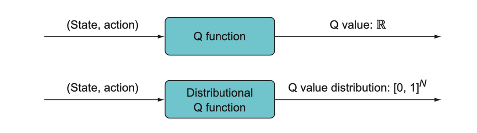
Most environments we wish to apply reinforcement learning to involve some amount of randomness or unpredictability, where the rewards we observe for a given state-action pair have some variance. In ordinary Q-learning, which we might call expected-value Q-learning, we only learn the average of the noisy set of observed rewards. Distributional Q-learning seeks to get a more accurate picture of the distribution of observed rewards.

Probability and statistics

The two major camps in probability theory are called frequentists and Bayesians.

Frequentist	Bayesian
Probabilities are frequencies of individual outcomes	Probabilities are degrees of belief
Computes the probability of the data given a model	Computes the probability of a model given the data
Uses hypothesis testing	Uses parameter estimation or model comparison
Is computationally easy	Is (usually) computationally difficult

Priors and posteriors

In the Bayesian framework, probabilities represent beliefs, and beliefs are always tentative in situations when new information can become available, so a prior probability distribution is just the distribution you start with before receiving some new information. After some new information is received, the updated distribution is now called the posterior probability distribution.

The beliefs are continually updated as a succession of prior distributions to posterior distributions, and this process is generically called Bayesian inference.

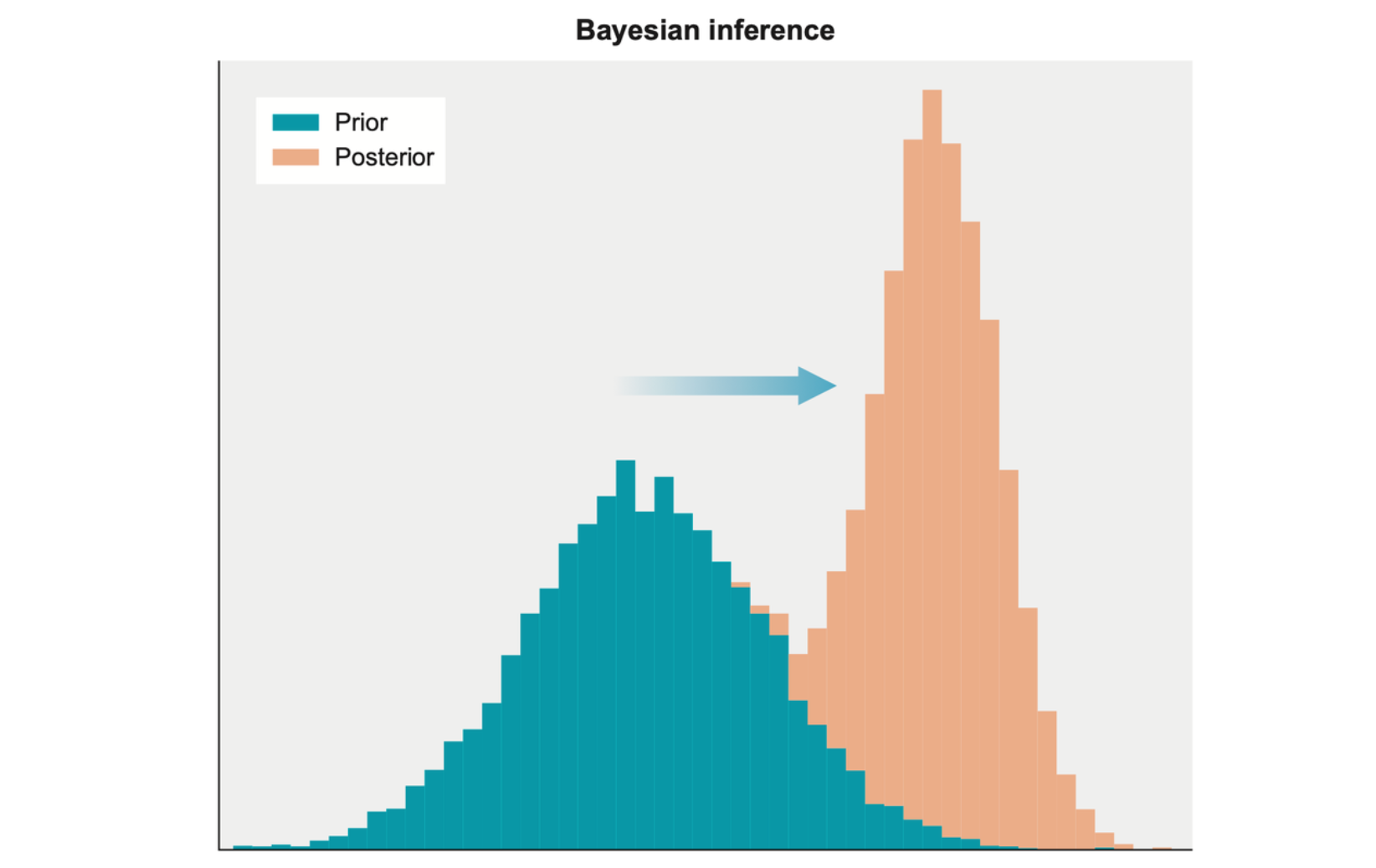
Bayesian inference is the process of starting with a prior distribution, receiving some new information, and using that to update the prior into a new, more informed distribution called the posterior distribution.

Bayesian inference is the process of starting with a prior distribution, receiving some new information, and using that to update the prior into a new, more informed distribution called the posterior distribution.

The Bellman equation

The Bellman equation tells us how to update the Q function when rewards are observed.

\[ Q_\pi(s_t, a_t) \gets r_t + \gamma \cdot V_\pi(s_{t+1}) \]

where \(V_\pi(s_{t+1}) = \max [Q_\pi(s_{t+1}, a)]\). If we use neural networks to approximate the Q function, we try to minimize the error between the predicted \(Q_\pi(s_t, a_t)\) on the left side of the Bellman equation and the quantity on the right side by updating the neural network’s parameters.

The distributional Bellman equation

The Bellman equation implicitly assumes that the environment is deterministic and thus that observed rewards are deterministic (i.e. the observed reward will be always the same if you take the same action in the same state). But sometimes some amount of randomness is involved. In this case, we can make the deterministic variable \(r_t\) into a random variable \(R(s_t, a)\) that has some underlying probability distribution. If there is randomness in how states evolve into new states, the Q function must be a random variable as well. The original Bellman equation can now be represented as

\[ Q(s_t, a_t) \gets \mathbb{E}[R(s_t, a)] + \gamma \cdot \mathbb{E}[Q(S_{t+1}, A_{t+1})] \]

If we get rid of the expectation operator, we get a full distributional Bellman equation:

\[ Z(s_t, a_t) \gets R(s_t, a) + \gamma \cdot Z(S_{t+1}, A_{t+1}) \]

Here we use \(Z\) to denote the distributional Q value function (which will also be referred to as the value distribution).

Distributional Q-learning

Representing a probability distribution in Python

A discrete probability distribution over rewards can be represented by two numpy arrays. One numpy array will be the possible outcomes, and the other will be an equal-sized array storing the probabilities for each associated outcome.

Though \(Z(s, a)\) should not be restricted by the outcome range, our array have to be limited by a minimum and maximum value.

In Dist-DQN learning, we use whatever distribution the Dist-DQN returns for the subsequent state, \(s_{t+1}\), as a prior distribution, and we update the prior distribution with the single observed reward, \(r_t\), such that a little bit of the distribution gets redistributed around the observed \(r_t\).

This figure shows how a uniform distribution changes with lower or higher values for gamma (the discount factor)

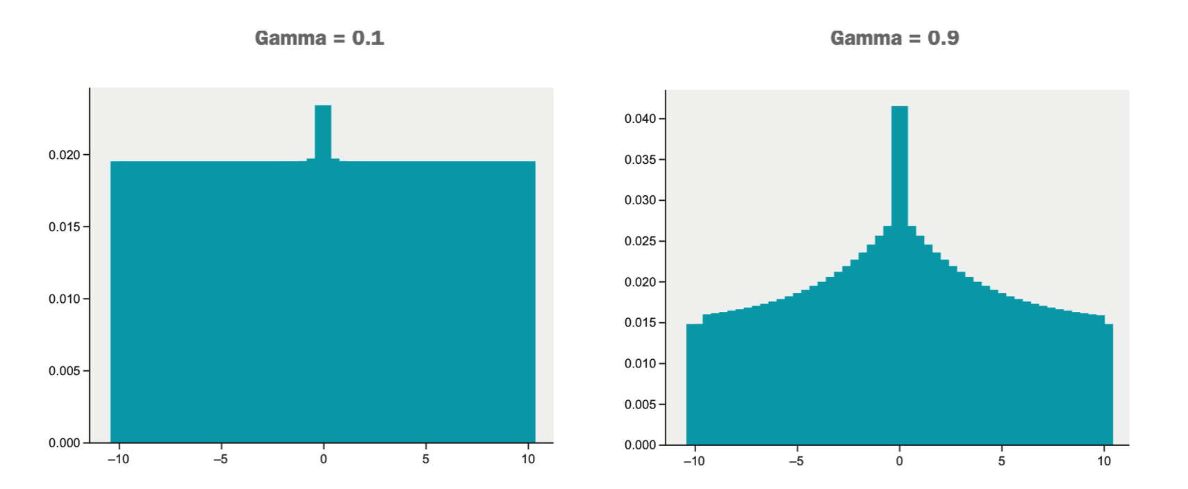
This figure shows how a uniform distribution changes with lower or higher values for gamma (the discount factor)

Once we have the distribution, we have

\[ \mathrm{d}z = \frac{v_{\max} - v_{\min}}{N - 1} \]

as the “bar width”, then we can use it to find the closest support element index value by

\[ b_j = \bigg\lfloor\frac{r - v_{\min}}{\mathrm{d}z}\bigg\rfloor \]

as the “bar index”, where \(r\) is the reward.

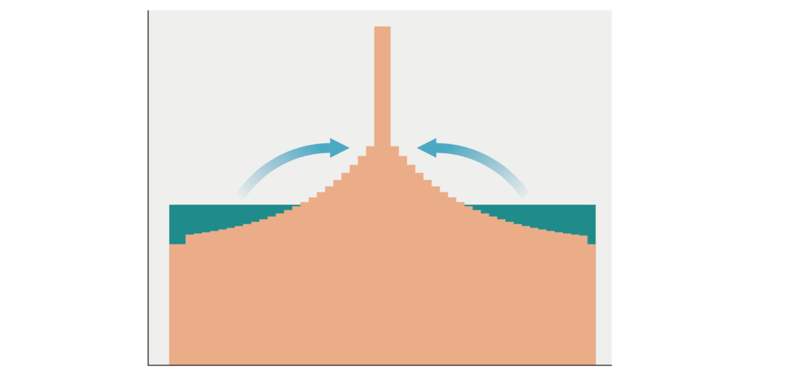
Once we find the index value of the support element corresponding to the observed reward, we want to redistribute some of the probability mass to that support and the nearby support elements. We will simply take some of the probability mass from the neighbors on the left and right and add it to the element that corresponds to the observed reward.

The update_dist function redistributes probability from neighbors toward the observed reward value.

def update_dist(r, support, probs, lim=(-10., 10.), gamma=0.8):
    nsup = probs.shape[0]
    vmin, vmax = lim[0], lim[1]
    dz = (vmax - vmin) / (nsup - 1.)
    bj = np.round((r - vmin) / dz)
    bj = int(np.clip(bj, 0, nsup - 1))
    m = probs.clone()
    j = 1
    for i in range(bj, 1, -1):
        m[i] += np.power(gamma, j) * m[i - 1]
        j += 1
    j = 1
    for i in range(bj, nsup - 1, 1):
        m[i] += np.power(gamma, j) * m[i - 1]
        j += 1
    m /= m.sum()
    return m

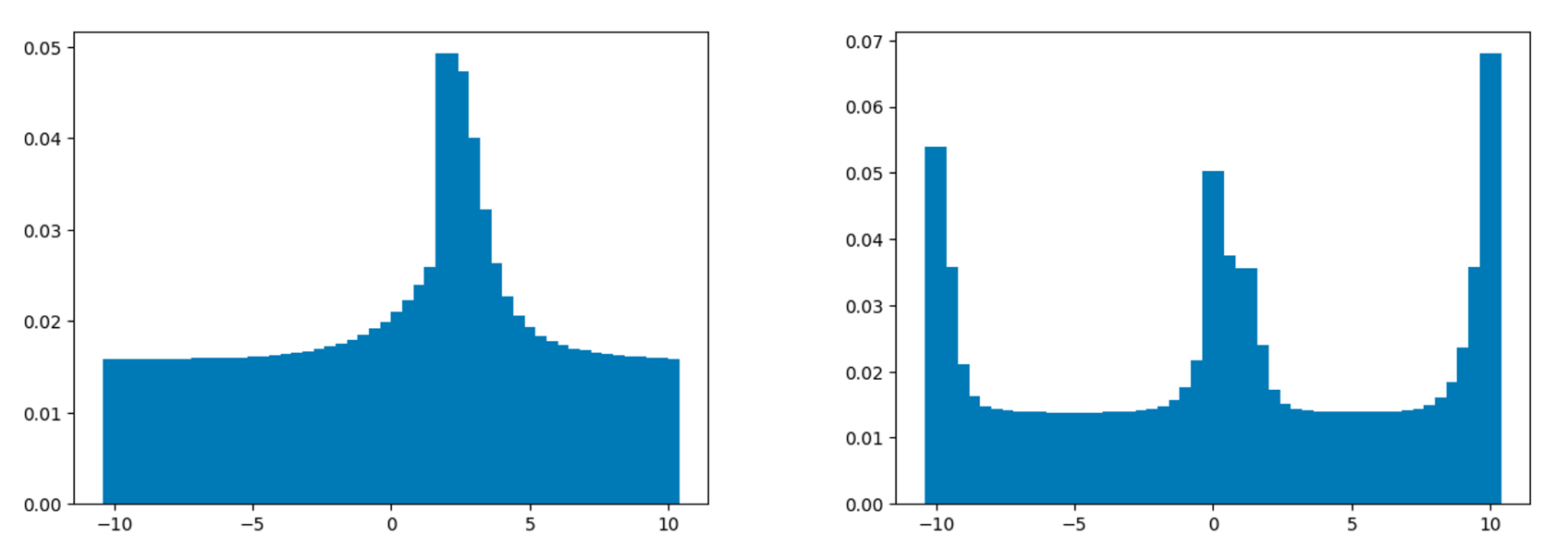
The left graph shows the distribution after a 2 reward is received. The right graph shows the distribution update can actually expressed the 2-modal distribution.

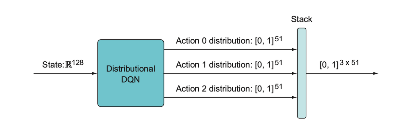
Implementing the Dist-DQN

In the game Freeway, the Dist-DQN will take a 128-element state vector, pass it through a couple of dense feedforward layers, and then it will use a for loop to multiply the last layer by 3 separate matrices to get 3 separate distribution vectors. (Since in game Freeway there are 3 actions).

Then we collect these 3 output distributions into a single 3 x 51 matrix and return that as the final output of the Dist-DQN. Thus, we can get the individual action-value distributions for a particular action by indexing a particular row of the output matrix.

Summary

• The advantages of distributional Q-learning include improved performance and a way to utilize risk-sensitive policies.
• Prioritized replay can speed learning by increasing the proportion of highly informative experiences in the experience replay buffer.
• The Bellman equation gives us a precise way to update a Q function.
• The OpenAI Gym includes alternative environments that produce RAM states, rather than raw video frames. The RAM states are easier to learn since they are usually of much lower dimensionality.
• Random variables are variables that can take on a set of outcomes weighted by an underlying probability distribution.
• The entropy of a probability distribution describes how much information it contains.
• The KL divergence and cross-entropy can be used to measure the loss between two probability distributions.
• The support of a probability distribution is the set of values that have nonzero probability.
• Quantile regression is a way to learn a highly flexible discrete distribution by learning the set of supports rather than the set of probabilities.