Tackling more complex problems with actor-critic methods

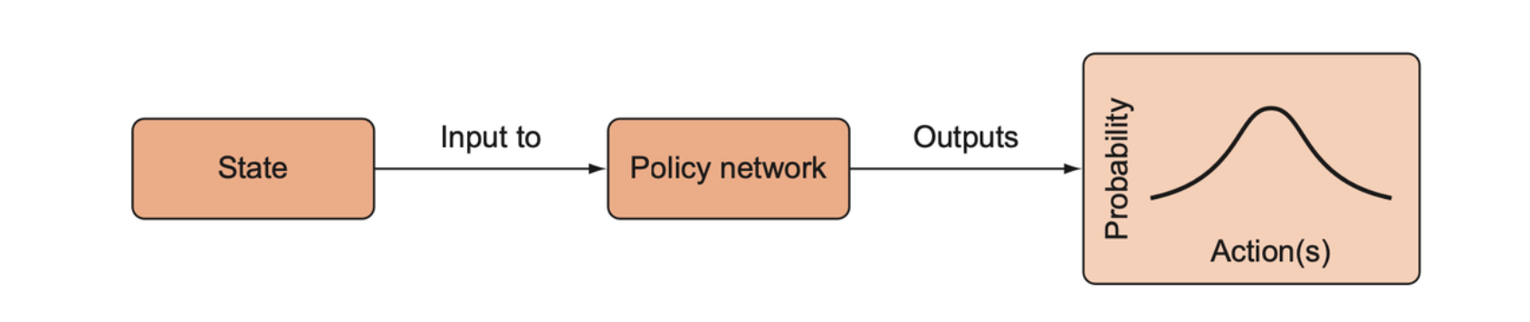
The REINFORCE algorithm is generally implemented as an episodic algorithm, meaning that we only apply it to update our model parameters after the agent has completed an entire episode. The policy is a function, \(\pi: S \to P(a)\), it takes a state and returns a probability distribution over actions.

At the end of the episode, we compute the return of the episode, which is the sum of the discounted rewards in the episode. The return is calculated as

\[ R = \sum_t \gamma_t \cdot r_t \]

The loss function we minimize is defined as below

\[ \text{Loss} = -\log(P(a|S)) \cdot R \]

So with REINFORCE we just keep sampling episodes from the agent and environment, and periodically update the policy parameters by minimizing this loss. By sampling a full episode, we get a pretty good idea of the true value of an action because we can see its downstream effects rather than just its immediate effect. But not all environments are episodic, and sometimes we want to be able to make updates in an incremental or online faction.

Distributed advantage actor-critic (DA2C) is a new kind of policy gradient method that will have the online-learning advantages of DQN without a replay buffer. It will also have the advantages of policy methods where we can directly sample actions from the probability distribution over actions.

Combining the value and policy function

Q-learning uses a trainable function to directly model the value (the expected reward) of an action, given a state. On the other hand, the advantage of direct policy learning is that we get a true conditional probability distribution over actions, \(P(a|S)\), that we can directly sample from to take an action.

We can combine these two approaches to get the advantages of both. In building such a combined value-policy learning algorithm, we will start the policy learner as the foundation. There are two challenges we want to overcome to increase the robustness of the policy learner:

• We want to improve the sample efficiency by updating more frequently.
• We want to decrease the variance of the reward we used to update our model.

The idea behind a combined value-policy algorithm is to use the value learner to reduce the variance in the rewards that are used to train the policy. That is, instead of minimizing the REINFORCE loss that included direct reference to the observed return \(R\) from an episode, we instead add a baseline value such that the loss is now

\[ \text{Loss} = -\underbrace{\log(\pi(a|S))}_{\substack{\text{Log probability of} \\ \text{action given state}}} \cdot (R - \underbrace{V_\pi(S)}_{\substack{\text{state} \\ \text{value}}}) \]

The quantity \(R - V_\pi(S)\) is actually the advantage of taking action \(a\) under state \(S\).

Algorithms of this sort are called actor-critic methods, where “actor” refers to the policy, because that’s where the actions are generated, and “critic” refers to the value function, because that’s what tells the actor how good its actions are. Since we are using \(R - V_\pi(S)\) rather than just \(V(S)\), this is called advantage actor-critic.

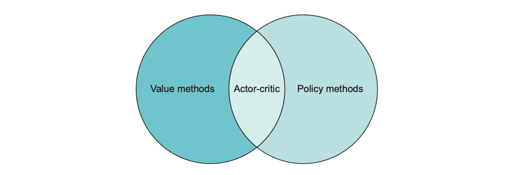
Q-learning falls under the category of value methods, since we attempt to learn action values, whereas policy gradient methods like REINFORCE directly attempt to learn the best actions to take. We can combine these two techniques into what’s called an actor-critic architecture.

💡 When we say an algorithm bootstraps, we mean it can make a prediction from a prediction.

Bootstrapping introduces a source of bias. Bias is a systematic deviation from the true value of something. On the other hand, making predictions from predictions introduces a kind of self-consistency that results in lower variance.

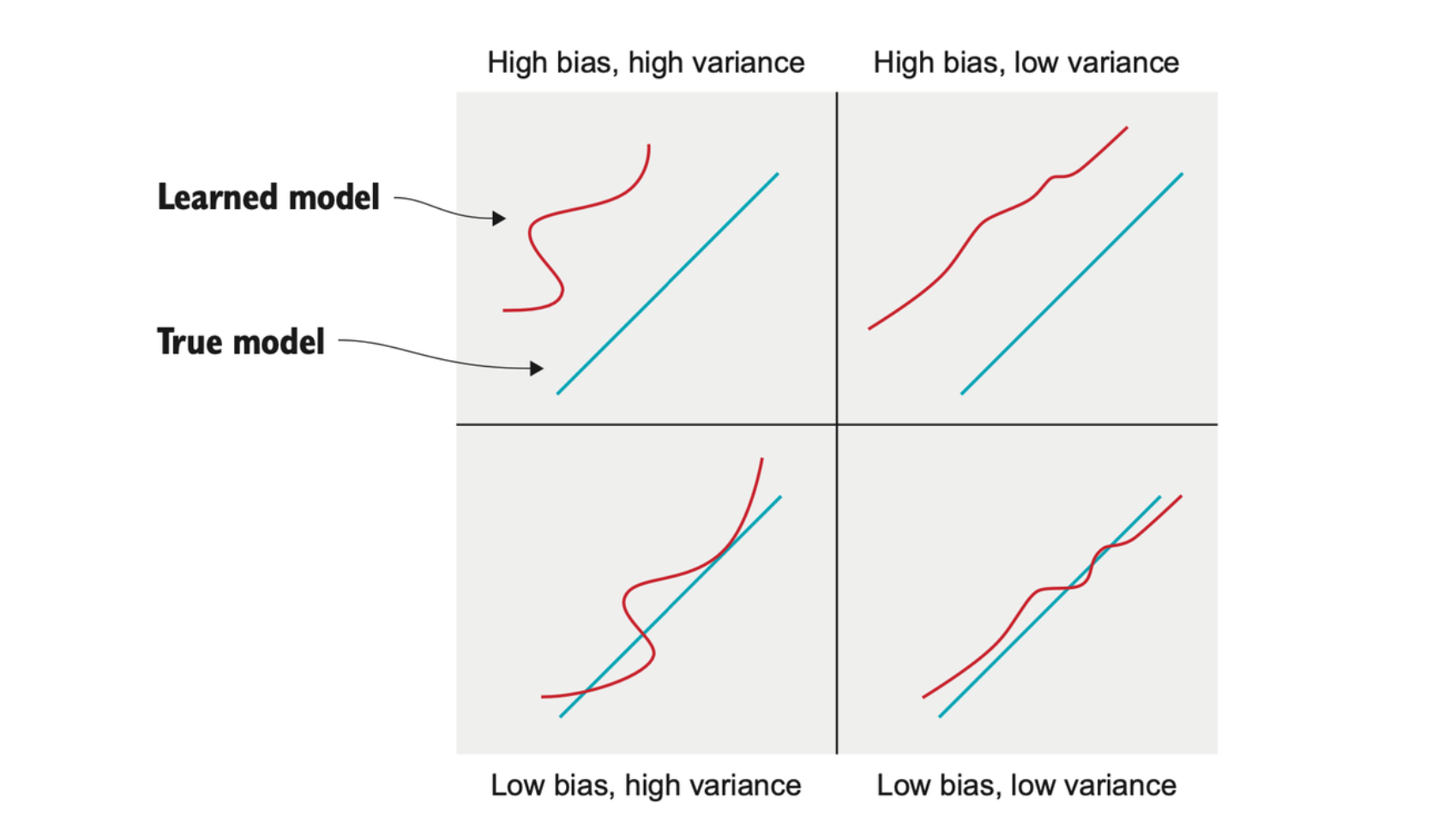
The bias-variance tradeoff is a fundamental machine learning concept that says any machine learning model will have some degree of systematic deviation from the true data distribution and some degree of variance. You can try to reduce the variance of your model, but it will always come at the cost of increased bias.

We want to combine the potentially high-bias, low-variance value prediction with the potentially low-bias, high-variance policy prediction to get something with moderate bias and variance —— something that will work well in the online setting.

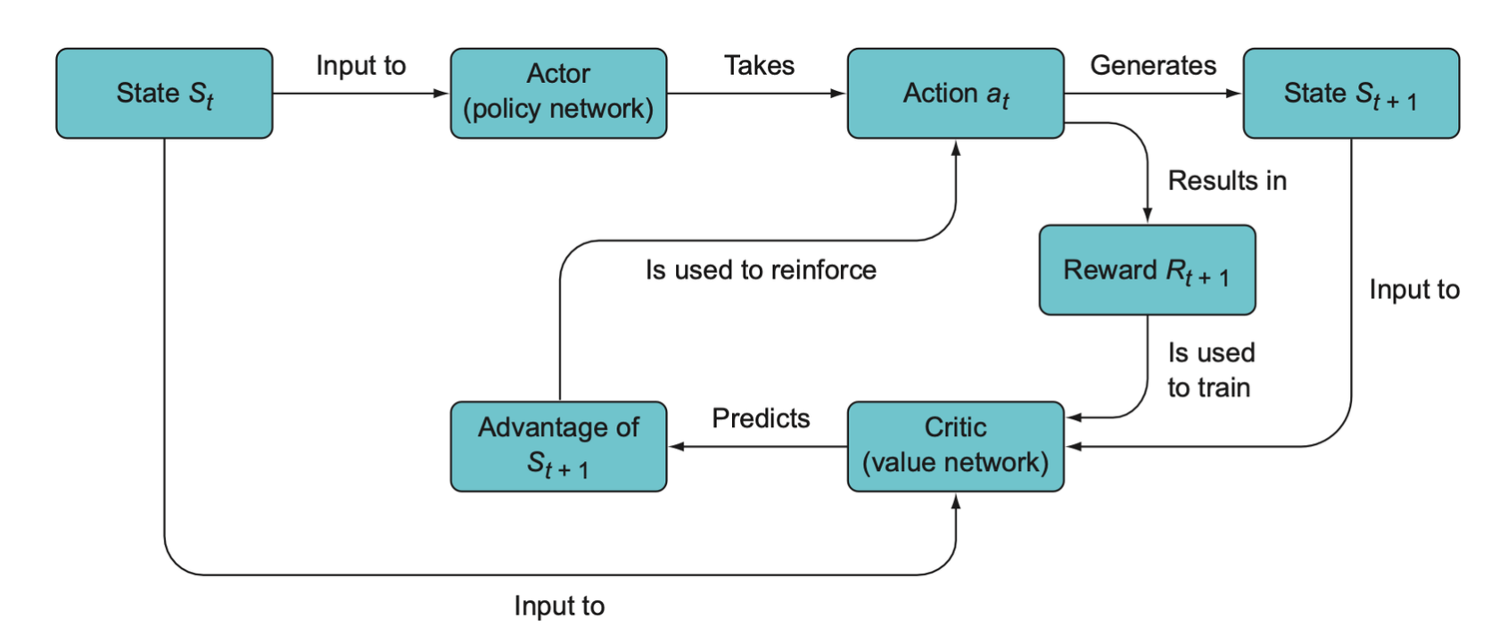
The general overview of actor-critic models. First, the actor predicts the best action and chooses the action to take, which generates a new state. The critic network computes the value of the old state and the new state. The relative value of \(S_{t+1}\) is called its advantage, and this is the signal used to reinforce the action that was taken by the actor.

Distributed training

Batch training is necessary because the gradients, if we trained with single pieces of data at a time, would have too much variance, and the parameters would never converge on their optimal values. We need to average out the noise in a batch of data to get the real signal before updating the model parameters.

This is why we had to use an experience replay buffer with DQN. Having a sufficiently large replay buffer requires a lot of memory, and in some cases a replay buffer is impractical.

In many complex games it is common to use recurrent neural networks like LSTM or GRU. These RNNs can keep an internal state that can store traces of the past. But experiences replay doesn’t work with an RNN unless the replay buffer stores entire trajectories or full episodes, because the RNN is designed to process sequential data.

One way to use RNNs without an experience replay is to run multiple copies of the agent in parallel, each with separate instantiations of the environment. By distributing multiple independent agents across different CPU processes, we can collect a varied set of experiences and therefore get a sample of gradients that we can average together to get a lower variance mean gradient.

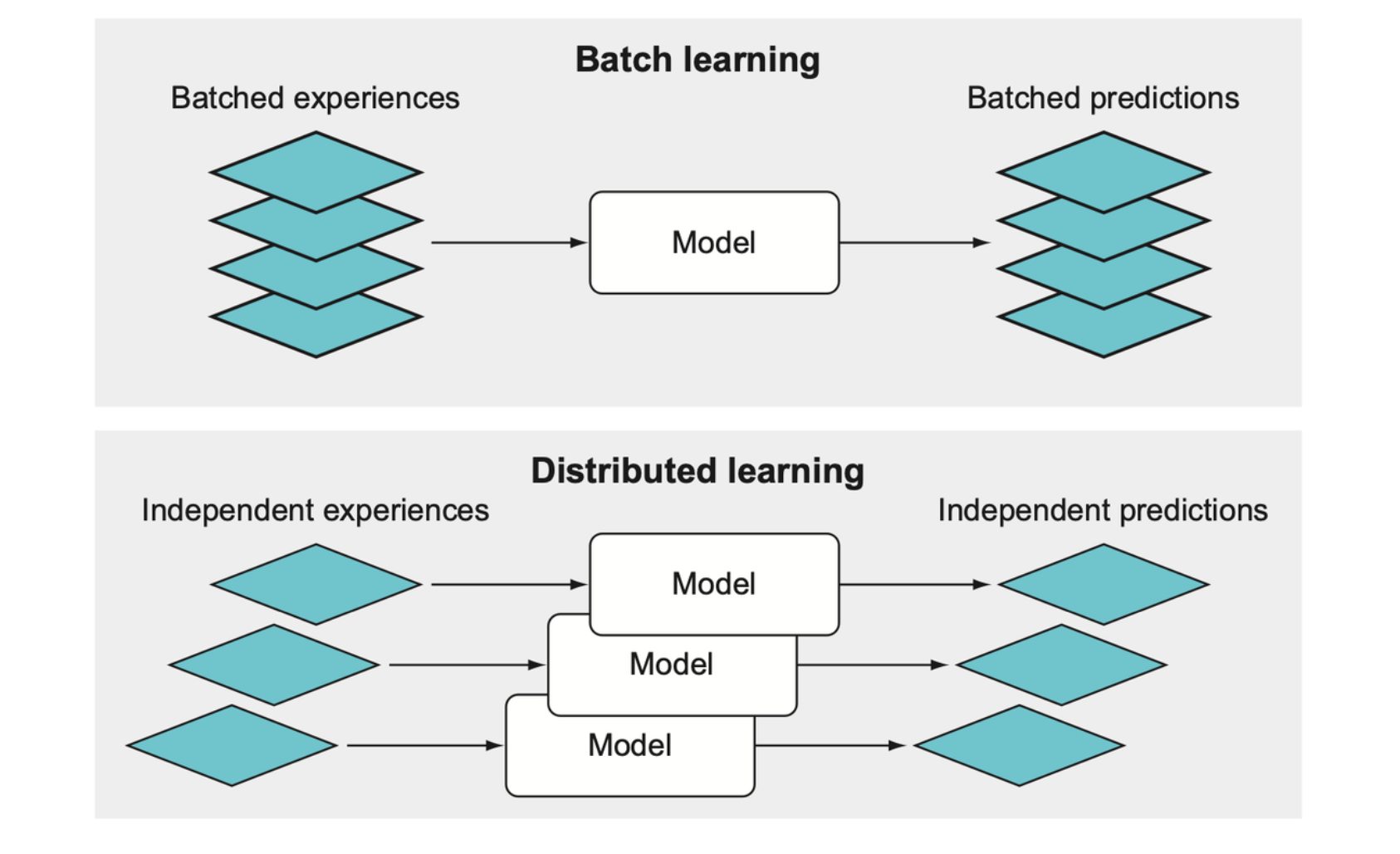
The most common form of training a deep learning model is to feed a batch of data together into the model to return a batch of predictions. Then we compute the loss for each prediction and average or sum all the losses before back-propagating and updating the model parameters. This averages out the variability present across all the experiences. Alternatively, we can run multiple models with each taking a single experience and making a single prediction, backpropagate through each model to get the gradients, and then sum or average the gradients before making any parameter updates.

Advantage actor-critic

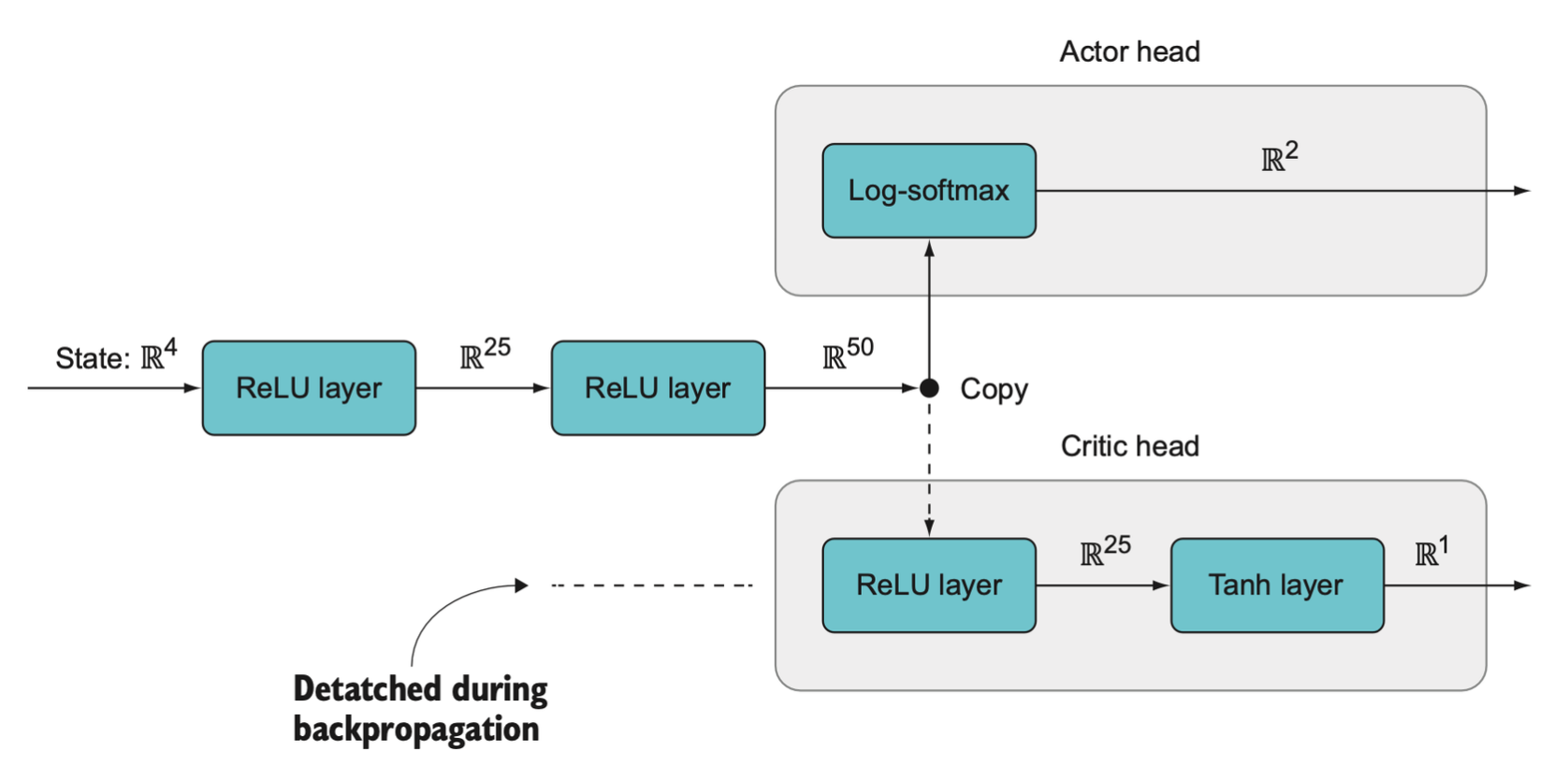
Though the actor and critic as two separate functions, but we can combine them into a single neural network with two output “heads”. The neural network will return two different vectors: one for the policy and one for the value. This allows for some parameter sharing between the policy and value that can make things more efficient, since some of the information needed to compute values is also useful for predicting the best action for the policy.

# pseudocode for online advantage actor-critic
gamma = 0.9
for i in epochs:
    state = environment.get_state()
    # predicts the value of the state
    value = critic(state)
    # predicts the probability distribution over actions given the state
    policy = actor(state)
    # sample an action
    action = policy.sample()
    next_state, reward = environment.take_action(action)
    # predicts the value of next state
    value_next = critic(next_state)
    advantage = reward + (gamma * value_next - value)
    loss = -1 * policy.logprob(action) * advantage
    minimize(loss)

The advantage function bootstraps because it computes a value for the current state and action based on predictions for a future state. The full advantage expression, \(A = r_{t+1} + \gamma \cdot v(s_{t + 1}) - v(s_t)\), is used when we do online or N-step learning.

N-step learning accumulate rewards over N steps and then compute our loss and back-propagate.

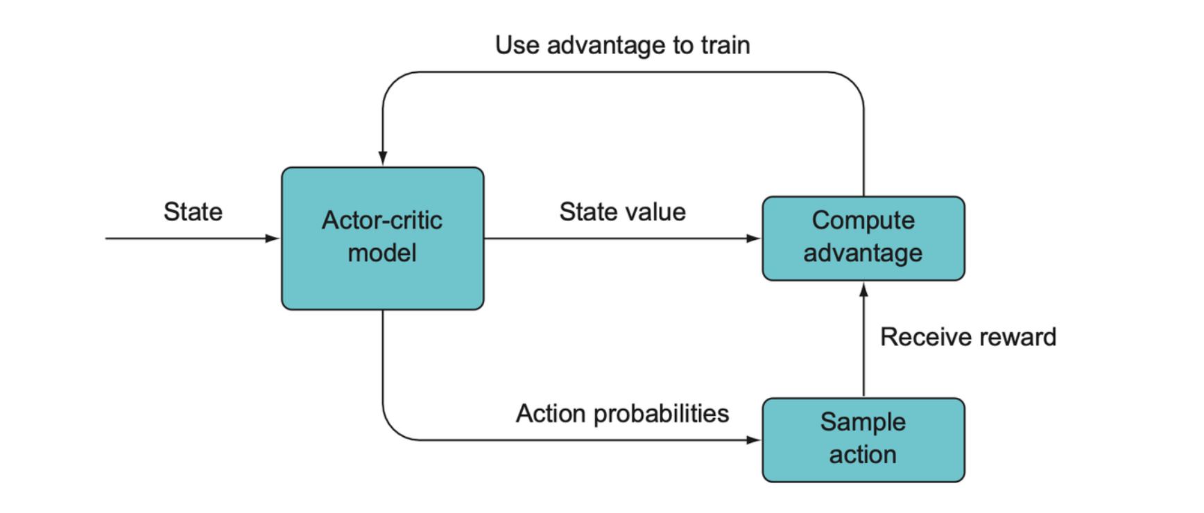
An actor-critic model produces a state value and action probabilities, which are used to compute an advantage value and this is the quantity that is used to train the model rather than raw rewards as with just Q-learning.

Coding an actor-critic model

1. Set up our actor-critic model, a two-headed model. The model accepts a state as input. The actor head is just like the policy network which produces a probability distribution over the actions. The critic outputs a single number representing the state value. The actor is denoted \(\pi(s)\) and the critic is denoted \(v(s)\).
2. While we’re in current episode
   1. Define the discount factor: \(\gamma\).
   2. Start a new episode, in initial state \(s_t\).
   3. Compute the value \(v(s_t)\) and store it in the list.
   4. Compute \(\pi(s_t)\), store it in the list, sample, and take action \(a_t\). Receive the new state \(s_{t+1}\)and the reward \(r_{t+1}\). Store the reward in the list.
3. Train
   1. Initialize \(R=0\). Loop through the rewards in reverse order to generate returns: \(R = r_i + \gamma \cdot R\).
   2. Minimize the actor loss: \(-1 \cdot \gamma_t \cdot (R - v(s_t)) \cdot \pi(a|s)\).
   3. Minimize the critic loss: \((R - v)^2\).
4. Repeat for a new episode.

Example for CartPole

This is an overview of the architecture for our two-headed actor-critic model. It has two shared linear layers and a branching point where the output of the first two layers is sent to a log-softmax layer of the actor head and also to a ReLU layer of the critic head before finally passing through a tanh layer, which is an activation function that restricts output between –1 and 1. This model returns a 2-tuple of tensors rather than a single tensor. Notice that the critic head is detached (indicated by the dotted line), which means we do not backpropagate from the critic head into the actor head or the beginning of the model. Only the actor back-propagates through the beginning of the model.

Within each process, an episode of the game is run using the shared model. The loss is computed within each process, but the optimizer acts to update the shared actor-critic model that is used by each process.

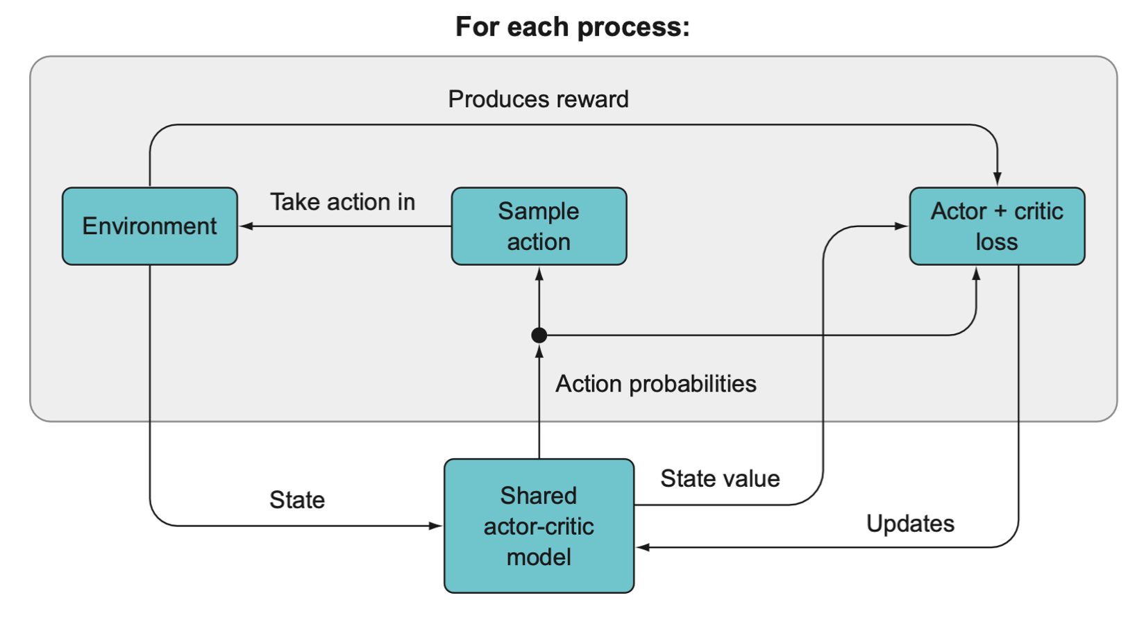
Each worker will update the shared model parameters asynchronously, whenever it is done running an episode.

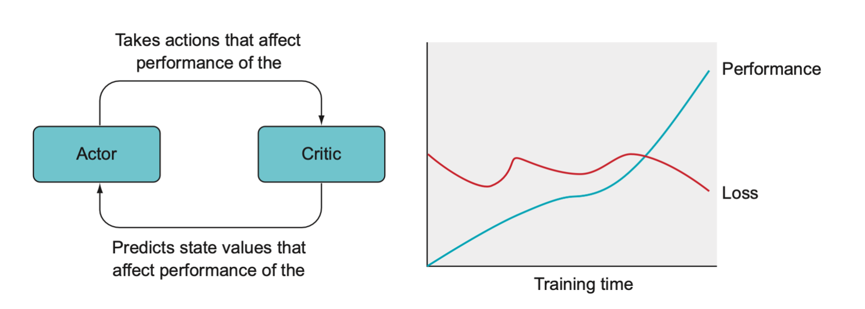
The actor and critic have a bit of an adversarial relationship since the actions that the agent take affect the loss of the critic, and the critic makes predictions of state values that get incorporated into the return that affects the training loss of the actor. Hence, the overall loss plot may look chaotic despite the fact that the agent is indeed increasing in performance.

💡 While using an adversarial training like this, the loss will be largely uninformative.

N-step actor-critic

In Monte Carlo method, we ran a full episode before updating the model parameters. While that makes sense for a simple game, usually we want to be able to make more frequent updates.

With Monte Carlo full-episode learning, we don’t take advantage of bootstrapping, since there’s nothing to bootstrap. But with 1-step online learning, a lot of bias may be introduced.

With bootstrapping, we’re making a prediction from a prediction, so the predictions will be better if you’re able to collect more data before making them. And we like bootstrapping because it improves sample efficiency.

Summary

• Q-learning learns to predict the discounted rewards given a state and action.
• Policy methods learn a probability distribution over actions given a state.
• Actor-critic models combine a Q-learner with a policy learner.
• Advantage actor-critic learns to compute advantages by comparing the expected value of an action to the reward that was actually observed, so if an action is expected to result in a –1 reward but actually results in a +10 reward, its advantage will be higher than an action that is expected to result in +9 and actually results in +10.
• Multiprocessing is running code on multiple different processors that can operate simultaneously and independently.
• Multithreading is like multitasking; it allows you to run multiple tasks faster by letting the operating system quickly switch between them. When one task is idle (perhaps waiting for a file to download), the operating system can continue working on another task.
• Distributed training works by simultaneously running multiple instances of the environment and a single shared instance of the DRL model; after each time step we compute losses for each individual model, collect the gradients for each copy of the model, and then sum or average them together to update the shared parameters. This lets us do mini-batch training without an experience replay buffer.
• N-step learning is in between fully online learning, which trains 1 step at a time, and fully Monte Carlo learning, which only trains at the end of an episode. N-step learning thus has the advantages of both: the efficiency of 1-step learning and the accuracy of Monte Carlo.