Learning to pick the best policy: Policy gradient methods

A Q-network takes a state and returns Q values (action values) for each action. We can use those action values to decide which actions to take.

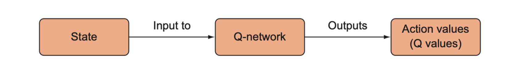
If we skip selecting a policy on top of the DQN and instead train a neural network to output an action directly, the network ends up being a policy function, or a policy network.

Policy function using neural networks

Instead of training a network that outputs action values, we will train a network to output (the probability of) actions.

Neural network as the policy function

In contrast to a Q-network, a policy network tells us exactly what to do given the state we’re in. All we need to do is randomly sample from the probability distribution \(P(A|S)\), and we get an action to take.

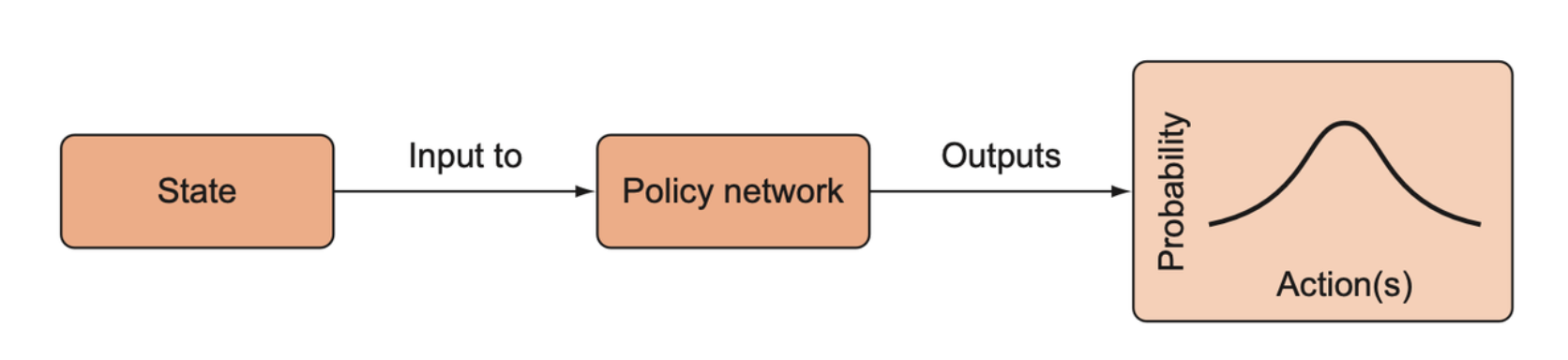
A policy network is a function that takes a state and returns a probability distribution over the possible actions.

Policy gradient methods offer a few advantages over value prediction methods like DQN.

• We no longer have to worry about devising an action-selection strategy like epsilon-greedy; instead, we directly sample actions from the policy.
• In order to improve the stability of training DQN, we had to use experience replay and target networks. A policy network tends to simplify some of that complexity.

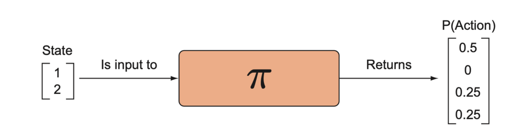
Stochastic policy gradient

A stochastic policy function. A policy function accepts a state and returns a probability distribution over actions. It is stochastic because it returns a probability distribution over actions rather than returning a deterministic, single action.

If the environment is stationary, which is when the distribution of states and rewards is constant, and we use a deterministic strategy, we’d expect the probability distribution to eventually converge to a degenerate probability distribution.

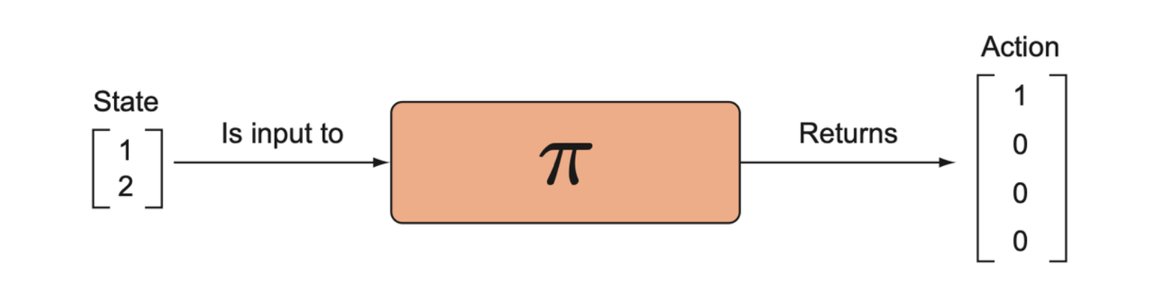
Early in training we want the distribution to be fairly uniform so that we can maximize exploration, but over the course of training we want the distribution to converge on the optimal actions, given a state.

Exploration

Since in stochastic policy gradient methods, the output is a probability distribution, there should be a small chance that we explore all spaces.

Building a notion of uncertainty into the models is generally a good thing.

Reinforcement good actions: The policy gradient algorithm

Defining an objective

With a policy network, we’re predicting actions directly, and there is not way to come up with a target vector of actions we should have taken instead, given the rewards. All we know is whether the action led to positive or negative rewards. In fact, what the best action is secretly depends on a value function, but with a policy network we’re trying to avoid computing these action values directly.

Keep using the policy network to generate action distribution, then select action until the end of an episode. We have a series of experience tuples.

\[ \varepsilon = (S_0, A_0, R_1), (S_1, A_1, R_2), \dots, (S_{t-1}, A_{t-1}, R_t) \]

If the reward is good, then the actions must have been “good” to some degree. Given the states we were in, we should encourage our policy network to make those actions more likely next time. We want to reinforce those actions that led to a nice positive reward.

Action reinforcement

The probability of an action, given the parameters of the policy network, is denoted \(\pi_s(a|\theta)\).

💡 This means we have some function that takes a parameter \(\theta\) and returns a probability distribution over some other parameter \(a\).

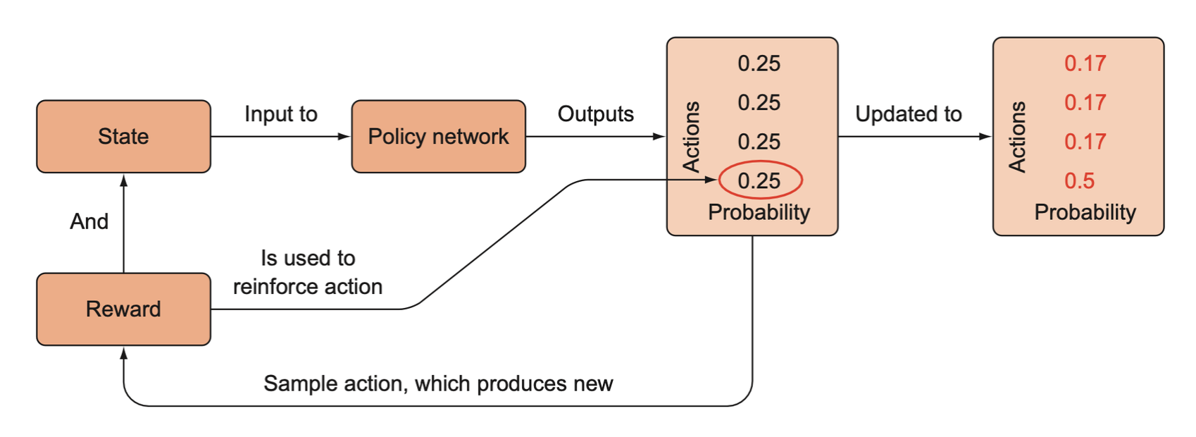
Once an action is sampled from the policy network’s probability distribution, it produces a new state and reward. The reward signal is used to reinforce the action that was taken, that is, it increases the probability of that action given the state if the reward is positive, or it decreases the probability if the reward is negative. Notice that we only received information about action 3 (element 4), but since the probabilities must sum to 1, we have to lower the probabilities of the other actions.

Log probability

The probabilities are bounded by 0 and 1 by definition, so the range of values that the optimizer can operate over is limited and small. Sometimes probabilities may be extremely tiny or very close to 1, and this runs into numerical issues when optimizing on a computer with limited numerical precision. If we use a surrogate objective, \(-\log \pi_s(a|\theta)\), we have an objective that has a larger “dynamic range” than raw probability space and this makes the log probability easier to compute.

Credit assignment

The last action right before the reward deserves more credit for winning the game than does the first action in the episode. Our confidence in how “good” each action is diminishes the further we are from the point of reward. This is the problem of credit assignment.

The final objective function that we will tell PyTorch to minimize is \(-\gamma_t G_t\log \pi_s(a|\theta)\), where \(\gamma_t\) is the discount factor. The parameter \(G_t\) is the total return. It is the return we expect to collect from time step \(t\) until the end of the episode, and it can be approximated by adding the rewards from some state in the episode until the end of the episode.

\[ G_t = r_t + r_{t+1} + \cdots + r_T \]

The discount is exponentially decayed from \(1\), \(\gamma_t = \gamma_0^{T - t}\). For example, if the agent is in state \(S_0\) and it takes action \(a_1\) and receives reward \(r_{t+1} = -1\), the target update will be \(-\gamma^0(-1)\log \pi(a_1 | \theta, S_0) = \log \pi(a_1 | \theta, S_0)\).

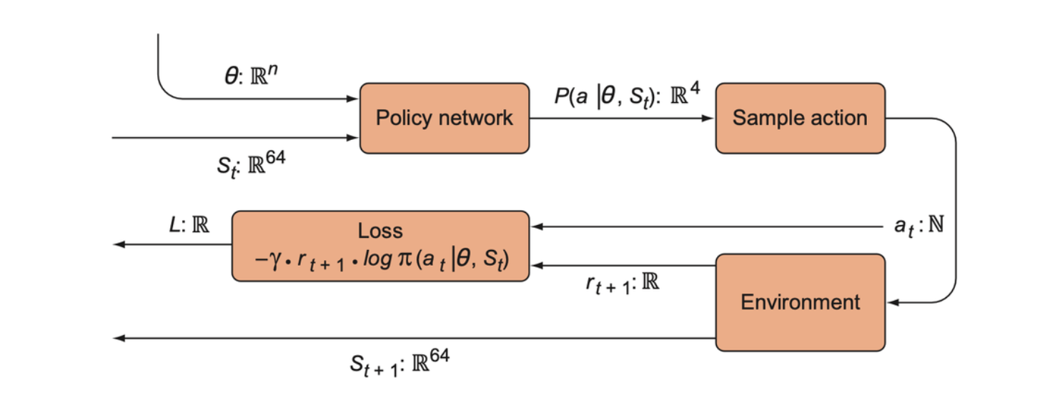
A string diagram for training a policy network for Grid world. The policy network is a neural network parameterized by \(\theta\) (the weights) that accepts a 64-dimensional vector for an input state. It produces a discrete 4-dimensional probability distribution over the actions. The sample action box samples an action from the distribution and produces an integer as the action, which is given to the environment (to produce a new state and reward) and to the loss function so we can reinforce that action. The reward signal is also fed into the loss function, which we attempt to minimize with respect to the policy network parameters.

The REINFORCE algorithm

Policy gradient focused on a particular algorithm that has been around for decades called REINFORCE.

Creating the policy network

The policy network is a neural network that takes state vectors as inputs, and it will produce a probability distribution over the possible actions.

import torch

l1 = 4   # size of state space is 4
l2 = 150 # hidden layer
l3 = 2   # size of action space

model = torch.nn.Sequential(
    torch.nn.Linear(l1, l2),
    torch.nn.LeakyReLU(),
    torch.nn.Linear(l2, l3),
    torch.nn.Softmax()
)

learning_rate = 0.0009
optimizer = torch.optim.Adam(model.parameters(), lr=learning_rate)

Having the agent interact with the environment

The agent consumes the state and takes an action, \(a\), probabilistically. The state is input to the policy network, which then produces the probability distribution over the actions \(P(A|\theta, S_t)\) given its current parameters and the state.

pred = model(torch.from_numpy(state1).float())
action = np.random.choice(np.array([0, 1]), p=pred.data.numpy())
state2, reward, terminated, truncated, info = env.step(action)

Training the model

We train the policy network by updating the parameters to minimize the objective function, this involves three steps:

1. Calculate the probability of the action actually taken at each time step.
2. Multiply the probability by the discounted return (the sum of rewards).
3. Use this probability-weighted return to backpropagate and minimize the loss.

Calculate the probability of the action

We can use the stored past transitions to recompute the probability distributions using the policy network, but this time we extract just the predicted probability for the action that was actually taken. This quantity is denoted as \(P(a_t|\theta, s_t)\). This is a single probability value.

To be concrete, let’s say the current state is \(S_5\). We input that into the policy network and it returns \(P_\theta(A|s_5) = [0.25, 0.75]\). We sample from this distribution and taken action \(a = 1\), and after this the pole falls over and the episode has ended. The total duration of the episode was \(T = 5\). For each of these 5 time steps, we took an action according to \(P_\theta(A|s_t)\) and we stored the specific probabilities of the actions that were actually taken, \(P_\theta(a|s_t)\) in an array, which might look like \([0.5, 0.3, 0.25, 0.5, 0.75]\). We simply multiply these probabilities by the discounted rewards, take the sum, multiply by -1, and call that our overall loss for this episode.

💡 Unlike Gridworld, in CartPole the last action is the one that loses the episode; we discount it the most since we want to penalize the worst move the most.

Minimizing this object function will tend to increase those probabilities \(P_\theta(a | s_t)\) weighted by the discounted rewards. Since probabilities must sum to 1, if we increase the probability of a good action, that will automatically steal probability mass from the other presumably less good actions.

Calculating future rewards

In the CartPole environment, if the episode lasted 5 time steps, the return array would be \([5, 4, 3, 2, 1]\). This makes sense because our first action should be rewarded the most, since it is the least responsible for the pole falling and losing the episode. To compute the discounted rewards, we can multiply the return array by discounted factors \([1, \gamma, \gamma^2, \gamma^3, \gamma^4]\).

def discount_rewards(rewards, gamma=0.99):
    lenr = len(rewards)
    disc_return = torch.pow(gamma, torch.arange(lenr).float()) * rewards
    # normalize rewards to be within [0, 1] to improve numerical stability
    disc_return /= disc_return.max()
    return disc_return

The loss function

The loss function is defined as above by the negative log-probability function. In PyTorch, this is defined as -1 * torch.sum(r * torch.log(preds)). We compute the loss with the data we’ve collected for the episode, and run the torch optimizer to minimize the loss.

The reason for this normalization step is to improve the learning efficiency and stability, since it keeps the return values within the same range no matter how big the raw return is.

def loss_fn(preds, r):
    return -1 * torch.sum(r * torch.log(preds))

Back-propagating

Since we have all the variables in our objective function, we can calculate the loss and backpropagate to adjust the parameters.

Summary

REINFORCE is an effective and very simple way of training a policy function, but it’s a little too simple. If we’re dealing with an environment with many more possible actions, reinforcing all of them each episode and hoping that on average it will only reinforce the good actions becomes less and less reliable.

• Probability is a way of assigning degrees of belief about different possible outcomes in an unpredictable process. Each possible outcome is assigned a probability in the interval \([0, 1]\) such that all probabilities for all outcomes sum to 1. If we believe a particular outcome is more likely than another, we assign it a higher probability. If we receive new information, we can change our assignments of probabilities.
• Probability distribution is the full characterization of assigned probabilities to possible outcomes. A probability distribution can be thought of as a function \(P: O \to [0, 1]\) that maps all possible outcomes to a real number in the interval \([0, 1]\) such that the sum of this function over all outcomes is 1.
• A degenerate probability distribution is a probability distribution in which only 1 outcome is possible (i.e., it has probability of 1, and all other outcomes have a probability of 0).
• Conditional probability is the probability assigned to an outcome, assuming you have some additional information (the information that is conditioned).
• A policy is a function, \(\pi: S \to A\), that maps states to actions and is usually implemented as a probabilistic function, \(\pi: P(A|S)\), that creates a probability distribution over actions given a state.
• The return is the sum of discounted rewards in an episode of the environment.
• A policy gradient method **is a reinforcement learning approach that tries to directly learn a policy by generally using a parameterized function as a policy function (e.g., a neural network) and training it to increase the probability of actions based on the observed rewards.
• REINFORCE is the simplest implementation of a policy gradient method; it essentially maximizes the probability of an action times the observed reward after taking that action, such that each action’s probability (given a state) is adjusted according to the size of the observed reward.