Predicting the best states and actions: Deep Q-networks

The Q function

The value function is defined as below, which is the weighted sum of all future rewards from the given state.

\[ V_\pi(s) = \sum^t_{i=1} w_i R_i = w_1 R_1 + w_2 R_2 + \cdots + w_t R_t \]

This weighted sum is an expected value and it’s often concisely denoted as \(E[R|\pi, s]\). Similarly, the action-value function \(Q_\pi(s, a)\) is denoted as \(E[R|\pi, s, a]\).

Navigate with Q-learning

Q-learning

Q-learning is a particular method of learning optimal action values, but there are other methods. The main idea of Q-learning is that your algorithm predicts the value of a state-action pair, and then you compare this prediction to the observed accumulated rewards at some later time and update the parameters of the algorithm, so that next time it will make better predictions.

\[ \overbrace{Q(S_t, A_t)}^\text{Updated Q value} = \overbrace{Q(S_t, A_t)}^\text{Current Q value} + \alpha[ \underbrace{R_{t+1}}_\text{Reward} + \gamma \underbrace{\max Q(S_{t+1}, a)}_\text{Max Q value for all actions} - Q(S_t, A_t) ] \]

where \(\alpha\) is learning rate and \(\gamma\) is discount factor.

Building the network

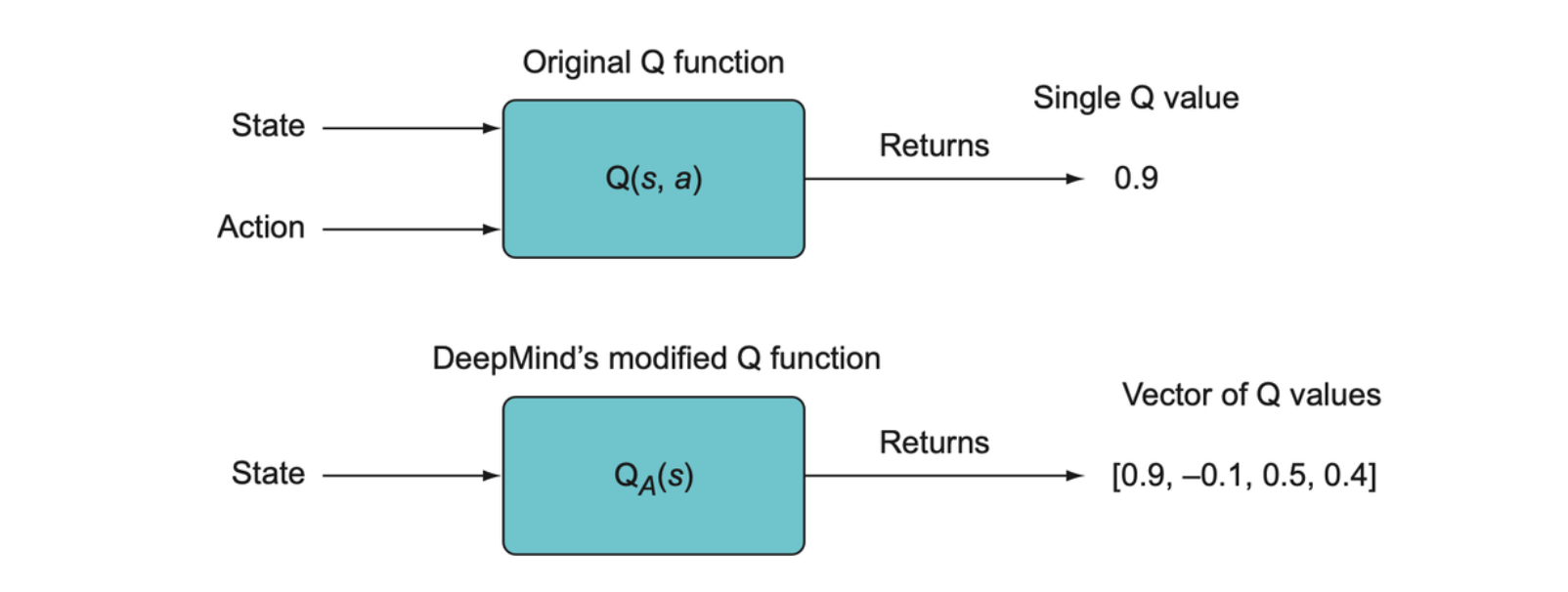
Generally, we want to use the Q function because it can tell us the value of taking an action in some state, so we can take the action that has the highest predicted value. But it would be rather wasteful to separately compute the Q values for every possible action given the state. A much more efficient procedure presented by DeepMind is to instead recast the Q function as a vector-valued function, it will compute the Q values for all actions, given some state, and return the vector of all those Q values. The new version of the Q function is denoted as \(Q_A(s)\).

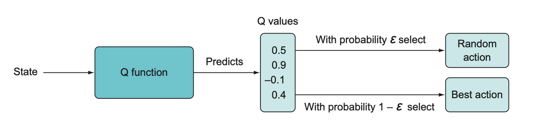
Once we have the output of the network, we can use it directly to decide what action to take using some action selection procedure, such as a simple epsilon-greedy approach or a softmax selection policy.

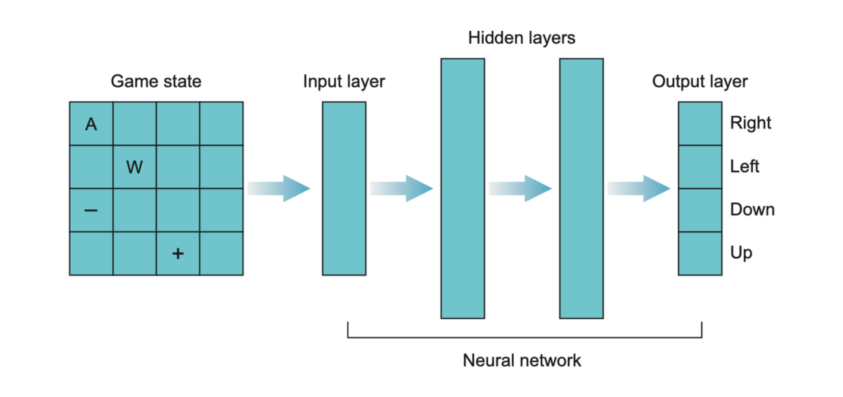
The whole neural network is shown as follows.

Learning process

1. Setup a for loop for the number of epochs.
2. In the loop, we setup a while loop (while the game is in progress).
3. Run the Q-network forward.
4. Using an epsilon-greedy implementation, so at time \(t\) with probability \(\varepsilon\) we will choose a random action. With probability \(1 - \varepsilon\), we will choose the action associated with the highest Q value from our network.
5. Take action \(a\) as determined in the preceding step, and observe the new state \(s'\) and reward \(r_{t + 1}\).
6. Run the network forward using \(s'\). Store the highest Q value, which we’ll call max Q.
7. Our target value for training the network is \(r_{t+1} + \gamma \max Q_A(S_{t+1})\). If after taking action \(a_t\) the game is over, there is no legitimate \(s_{t+1}\), we can set \(\gamma \max Q_A(S_{t+1})\) as 0. The target becomes just \(r_{t + 1}\).
8. Given that we have four outputs and we only want to update the output associated with the action we just took, our target output vector is the same as the output vector from the first run, except we change the one output associated with our action to the result we computed using the Q-learning formula.
9. Train the model on this one sample. Then repeat steps 2-9.

Preventing catastrophic forgetting: Experience replay

Catastrophic forgetting

It’s a very important issue associated with gradient descent-based training methods in online training.

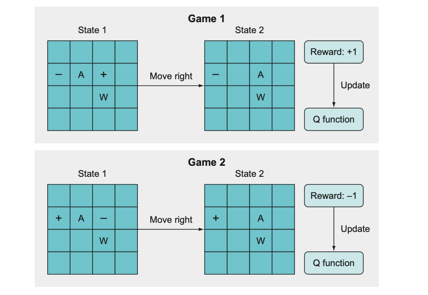
The idea of catastrophic forgetting is that when two game states are very similar and yet lead to very different outcomes, the Q function will get “confused” and won’t be able to learn what to do. In this example, the catastrophic forgetting happens because the Q function learns from game 1 that moving right leads to a +1 reward, but in game 2, which looks very similar, it gets a reward of –1 after moving right. As a result, the algorithm forgets what it previously learned about game 1, resulting in essentially no significant learning at all.

Experience replay

Experience replay basically gives us batch updating in an online learning scheme.

1. In state \(s\), take action \(a\), and observe the new state \(s_{t+1}\) and reward \(r_{t+1}\).
2. Store this as a tuple \((s, a, s_{t+1}, r_{t+1})\) in a list.
3. Continue to store each experience in this list until you have filled the list to a specific length.
4. Once the experience replay memory is filled, randomly select a subset.
5. Iterate through this subset and calculate value updates for each subset; store these in a target array (such as \(Y\)) and store the state, \(s\), of each memory in \(X\).
6. Use \(X\) and \(Y\) as a mini-batch for batch training. For subsequent epochs where the array is full, just overwrite old values in your experience replay memory array.

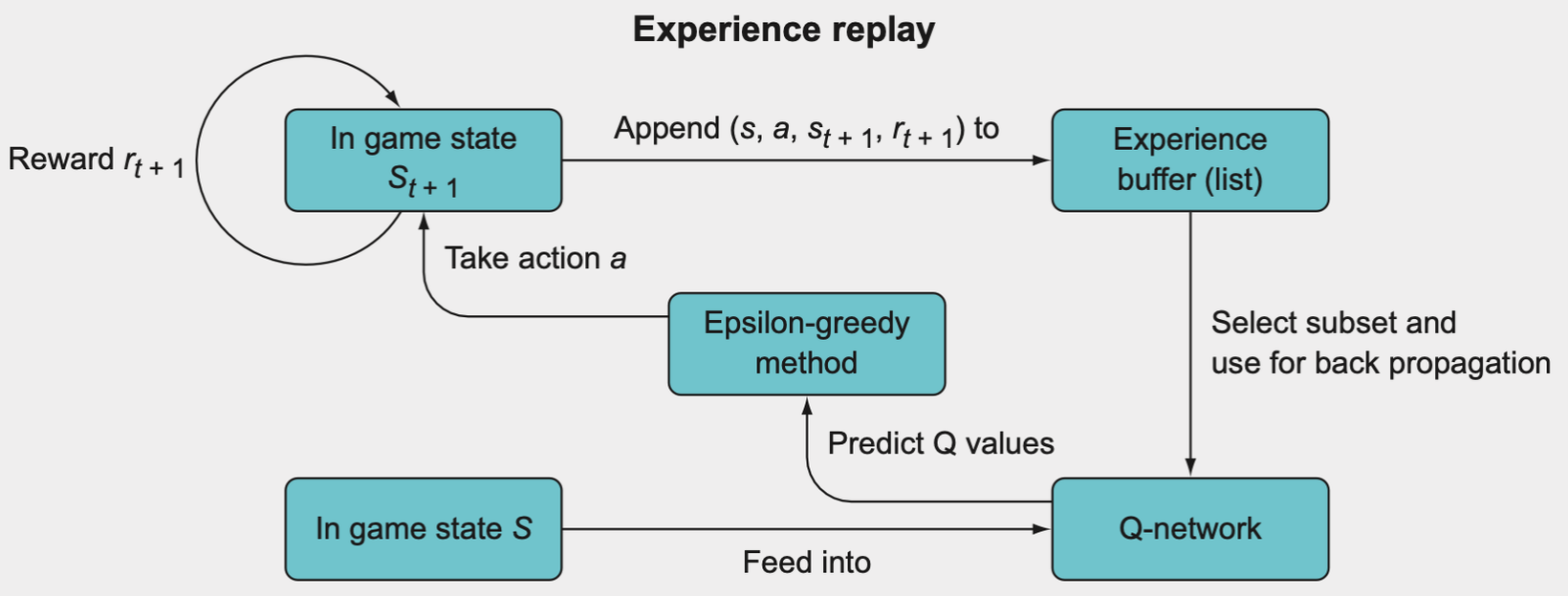
The idea is to employ mini-batching by storing past experiences and then using a random subset of these experiences to update the Q-network, rather than using just the single most recent experience.

Learning instability

One potential problem that DeepMind identified when they published their deep Q-network paper was that if you keep updating the Q-network’s parameters after each move, you might cause instabilities to arise. The idea is that since the reward may be sparse, updating on every single step, where most steps don’t get any significant reward, may cause the algorithm to start behaving erratically.

The solution is to duplicate the Q-network into two copies, each with its own model parameters. The regular Q-network and a copy called the target network.

The learning sequence is as follows:

1. Initialize the Q-network with parameters \(\theta_Q\).
2. Initialize the target network as a copy of the Q-network, but with separate parameters \(\theta_T\), and set \(\theta_T = \theta_Q\).
3. Use the epsilon-greedy strategy with the Q-network’s Q values to selection action \(a\).
4. Observe the reward and new state \(r_{t + 1}, s_{t+1}\).
5. The target network’s Q value will be set to \(r_{t+1}\) if the episode has just been terminated or to \(r_{t+1} + \gamma \max Q_{\theta_r}(S_{t+1})\) otherwise.
6. Backpropagate the target network’s Q value through the Q-network.
7. Every \(C\) number of iterations, set \(\theta_T = \theta_Q\).

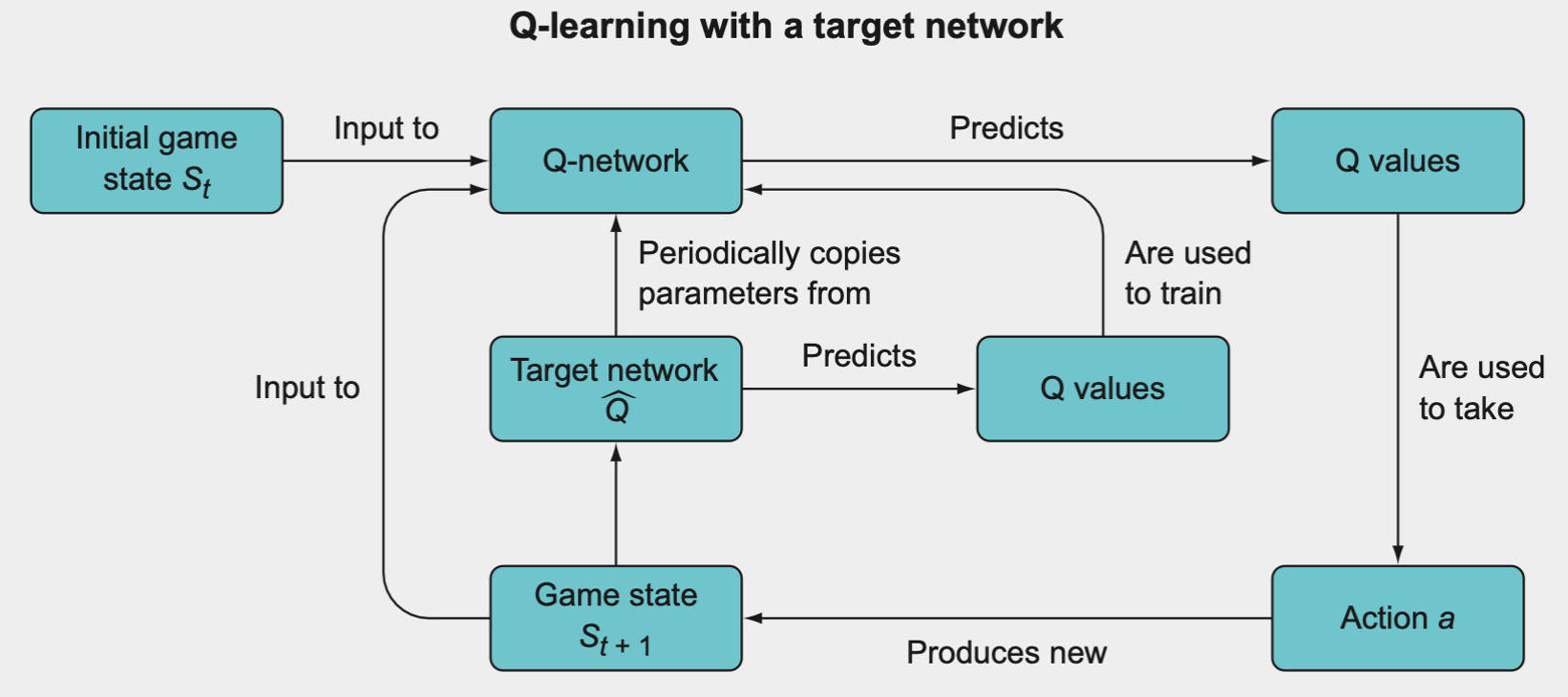
This is the general overview for Q-learning with a target network. It’s a fairly straightforward extension of the normal Q-learning algorithm, except that you have a second Q-network called the target network whose predicted Q values are used to backpropagate through and train the main Q-network. The target network’s parameters are not trained, but they are periodically synchronized with the Q-network’s parameters. The idea is that using the target network’s Q values to train the Q-network will improve the stability of the training.

Summary

• A state-space is the set of all possible states that the environment can be in. Usually the states are encoded as tensors, so the state space may be a vector of type \(\mathbb{R}^n\) or a matrix in \(\mathbb{R}^{n \times m}\).
• An action-space is the set of all possible actions given a state; for example, the action space for the game chess would be the set of all legal moves given some state of the game.
• A state-value is the expected sum of discounted rewards for a state given we follow some policy. If a state has a high state-value, that means that starting from this state will likely lead to high rewards.
• An action-value is the expected rewards for taking an action in a particular state. It is the value of a state-action pair. If you know the action-values for all possible actions for a state, you can decide to take the action with the highest action-value, and you would expect to receive the highest reward as a result.
• A policy function is a function that maps states to actions. It is the function that “decides” which actions to take given some input state.
• Q function **is a function that takes a state-action pair and returns the action-value.
• Q-learning is a form of reinforcement learning where we attempt to model the Q function; in other words, we attempt to learn how to predict the expected rewards for each action given a state.
• A deep Q-network (DQN) is simply where we use a deep learning algorithm as the model in Q-learning.
• Off-policy learning is when we learn a policy while collecting data using a different policy.
• On-policy learning **is when we learn a policy while also simultaneously using it to collect data for learning.
• Catastrophic forgetting is a big problem that machine learning algorithms face when training with small batches of data at a time, where the new data being learned erases or corrupts the old information already learned.
• Experience replay is a mechanism to allow batch training of reinforcement learning algorithms in order to mitigate catastrophic forgetting and allow stable training.
• A target network is a copy of the main DQN that we use to stabilize the update rule for training the main DQN.