More stable value-based methods

DQN: Making reinforcement learning more like supervised learning

Deep Q-network (DQN) is one of the most popular DRL algorithms because it started a series of research innovations that mark the history of RL.

Common problems in value-based deep reinforcement learning

Two most common problems in value-based deep reinforcement learning:

The violation of the IID assumption

In supervised learning, we obtain a full dataset in advance. We preprocess it, shuffle it, and then split it into sets for training. One crucial step in this process is the shuffling of the dataset. By doing so, we allow our optimization method to avoid developing overfitting biases.

In reinforcement learning, data is often gathered online; as a result, the experience sample generated at time step \(t+1\) correlates with experience sample gathered at time step \(t\). Moreover, as the policy is to improve, it changes the underlying data-generating process changes, which means that new data is locally correlated and not evenly distributed.

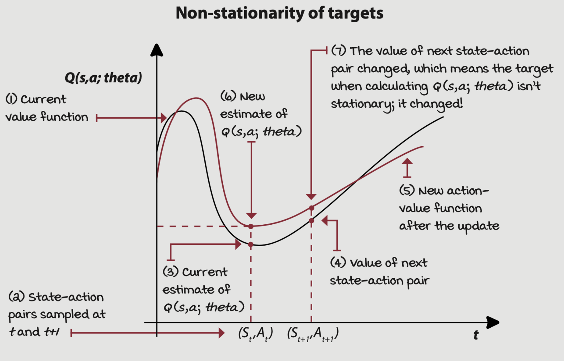
Stationary of targets

The targets we use to train our network are calculated using the network itself. As a result, the function changes with every update, in turn changing the targets.

Using target networks

A straightforward way to make target values more stationary is to have a separate network that we can fix for multiple steps and reserve it for calculating more stationary targets. The network with this purpose in DQN is called the target network.

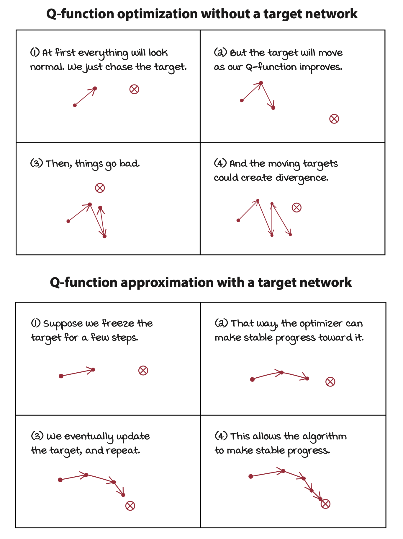
By using a target network to fix targets, we mitigate the issue of “chasing your own tail” by artificially creating several small supervised learning problems presented sequentially to the agent.

\[ \begin{gather} \nabla_{\theta_i} L_i(\theta_i) = \Bbb E_{s, a, r, s'}[(r + \gamma \max_{a'} Q(s', a'; \theta_i) - Q(s, a; \theta_i)) \nabla_{\theta_i} Q(s, a; \theta_i)] \\ \downarrow \\ \nabla_{\theta_i} L_i(\theta_i) = \Bbb E_{s, a, r, s'}[(r + \gamma \max_{a'} Q(s', a'; \textcolor{blue}{\theta^-}) - Q(s, a; \theta_i)) \nabla_{\theta_i} Q(s, a; \theta_i)] \end{gather} \]

The only difference between these two equations is the age of the neural network weights. A target network is a previous instance of the neural network that we freeze for a number of steps. In practice, we don’t have two “networks”, we have two instances of the neural network weights.

By using target networks, we stablize training, but we also slow down learning because you’re no longer training on up-to-date values.

Using larger networks

Another way to lessen the non-stationarity issue, to some degree, is to use larger networks.

💡 To mitigate the non-stationary issue we can 1. Create a target network that provides us with a temporarily stationary target value. 2. Create large-enough networks so that they can “see” the small differences between similar states (like those temporally correlated)

Using experience replay

Experience replay consists of a data structure, often referred to as a replay buffer or a replay memory, that holds experience samples for several steps, allowing the sampling of mini-batches from a broad set of past experiences.

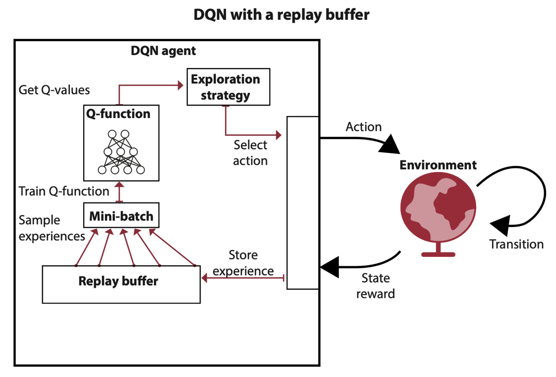
Unfortunately, the implementation becomes a little bit of challenge when working with high-dimensional observations, because poorly implemented replay buffers hit a hardware memory limit quickly in high-dimensional environments.

\[ \begin{gather} \nabla_{\theta_i} L_i(\theta_i) = \Bbb E_{s, a, r, s'}[(r + \gamma \max_{a'} Q(s', a'; {\theta^-}) - Q(s, a; \theta_i)) \nabla_{\theta_i} Q(s, a; \theta_i)] \\ \downarrow \\ \nabla_{\theta_i} L_i(\theta_i) = \Bbb E_{\textcolor{blue}{(s, a, r, s') \sim U(D)}}[(r + \gamma \max_{a'} Q(s', a'; {\theta^-}) - Q(s, a; \theta_i)) \nabla_{\theta_i} Q(s, a; \theta_i)] \end{gather} \]

The only difference between these two equations is that we’re now obtaining the experiences we use for training by sampling uniformly at ranom the replay buffer \(D\), instead of using the online experiences as before.

💡 The best solution to the problem of data not being IID is called experience replay. As the agent collects experiences tuples \(e_t = (S_t, A_t, R_{t+1}, S_{t+1})\) online, we insert them into a data structure, commonly referred to as the replay buffer \(D\), such that \(D = \{e_1, e_2, \dots, e_t\}\). The size of the replay buffer depends on the problem. Then the agent is trained on mini-batches sampled, usually uniformly at random, from the buffer, so that each sample has equal probability of being selected.

The full deep Q-network (DQN) algorithm

Selections we made

• Approximate the action-value function \(Q(s, a; \theta)\)
• Use a state-in-values-out architecture (nodes: 4, 512, 128, 2)
• Optimize the action-value function to approximate the optimal action-value function \(q^*(s, a)\)
• Use off-policy TD targets \((r + \gamma * \max_a' Q(s', a'; \theta))\) to evaluate policies
• Use MSE for loss function
• Use RMSprop as the optimizer with a learning rate of 0.0005

Some of the differences are that in the DQN implementation we now

• Use an exponentially decaying epsilon-greedy strategy to improve policies, decaying from \(1.0\) to \(0.3\) in roughly \(20,000\) steps.
• Use a replay buffer with \(320\) samples min, \(50,000\) max, and mini-batches of \(64\).
• Use a target network that updates every \(15\) steps.

DQN has three main steps:

1. Collect experiences tupes \((s, a, r, s', d)\) and insert it into the replay buffer
2. Randomly sample a mini-batch from the buffer, and calculate the off-policy TD targets \((r + \gamma * \max_{a'} Q(s', a'; \theta))\) for the whole batch
3. Fit the action-value function \(Q(s, a;\theta)\) using MSE and RMSprop

Double DQN: Mitigating the overestimation of action-value functions

One of the main improvements to DQN is called double deep Q-networks (DDQN). This improvement consists of adding double learning to our DQN agent.

Separating action selection from action evaluation

One way to better understand positive bias and how we can address it when using function approximation is by unwrapping the \(**\max**\) operator in the target calculations. The \(\max\) of a Q-function is the same as the Q-function of the \(\arg\max\) action.

\[ \max_{a'} Q(s', a'; \theta^-) \iff Q(s', \arg\max_{a'} Q(s', a'; \theta^-); \theta^-) \]

plugging this equivalence into the DQN function, we have

\[ \nabla_{\theta_i} L_i(\theta_i) = \Bbb E_{ {(s, a, r, s') \sim U(D)} }[(r + \gamma \textcolor{blue}{Q(s', \arg\max_{a'} Q(s', a'; \theta^-); \theta^-)} - Q(s, a; \theta_i)) \nabla_{\theta_i} Q(s, a; \theta_i)] \]

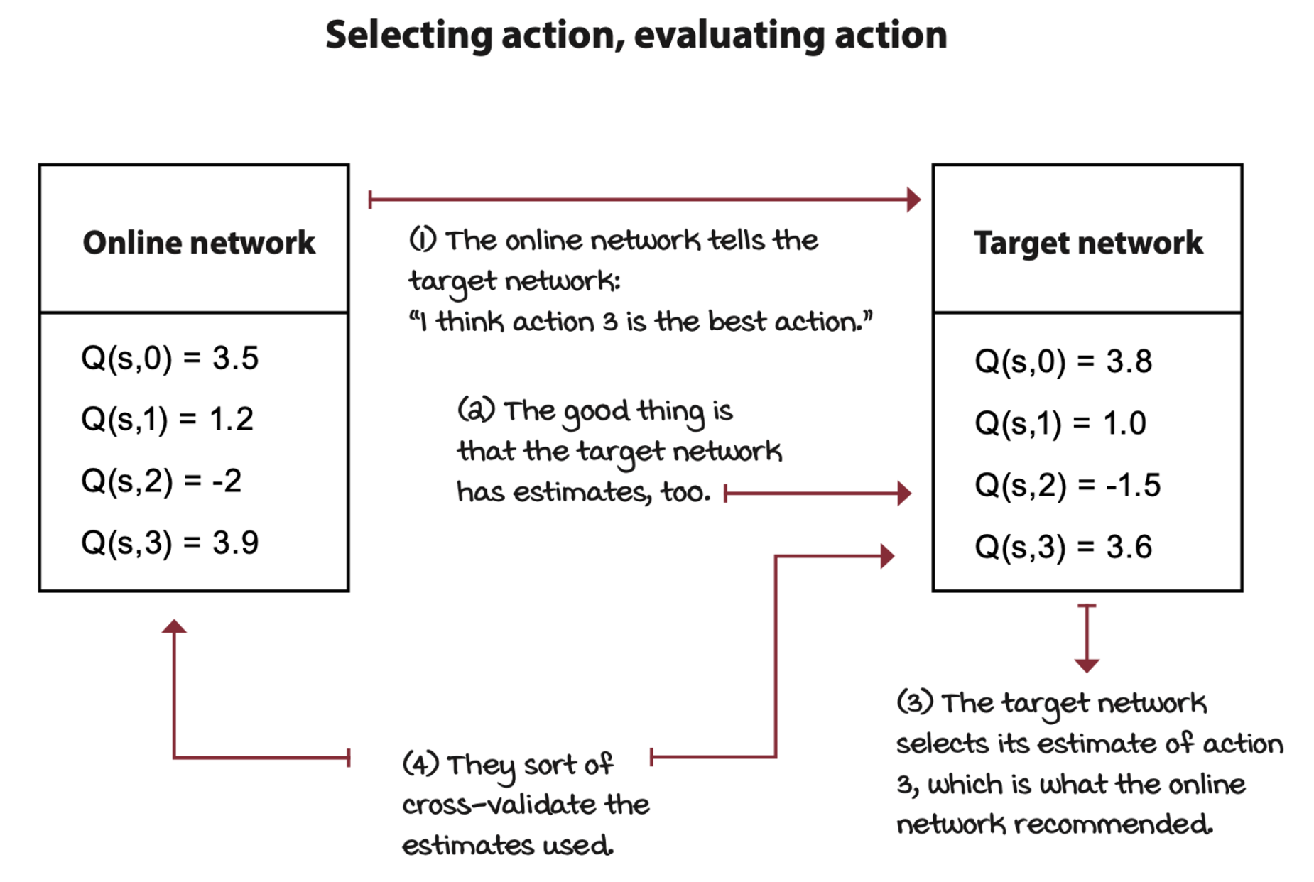
A way to reduce the chance of positive bias is to have two instances of the action-value function. In double learning, one estimator selects the index of what is believes to be the highest-valued action, and the other estimator gives the value of this action.

In practice, we can perform double learning with the other network, the target network. However, instead of training both the online and target networks, we continue training only the online network, but use the target network to help us cross-validate the estimates. We use the online network to find the index of the best action, then we use the target network to evaluate the previously selected action.

\[ \nabla_{\theta_i} L_i(\theta_i) = \Bbb E_{ {(s, a, r, s') \sim U(D)} }[(r + \gamma \textcolor{blue}{Q(s', \arg\max_{a'} Q(s', a'; \textcolor{red}{\theta_i}); \theta^-)} - Q(s, a; \theta_i)) \nabla_{\theta_i} Q(s, a; \theta_i)] \]

The only difference in DDQN is now we use the online weights to select the action, but still use the frozen weights to get the estimates.

A more forgiving loss function

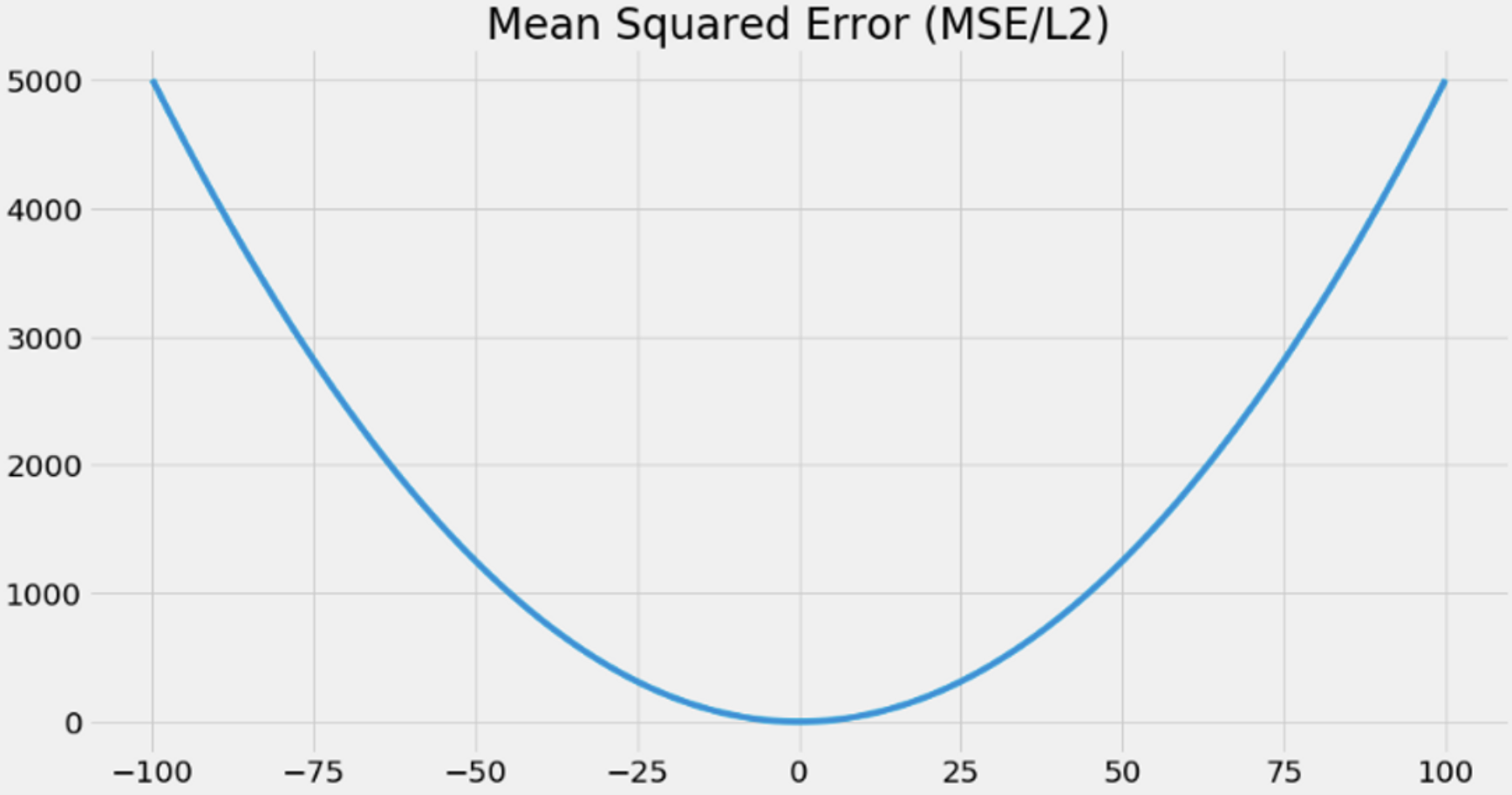
MSE is a ubiquitous loss fucntion because it’s simple, but one of the issues with using MSE for reinforcement learning is that it penalizes large errors more than small errors.

A more robust to outliers is the mean absolute error, also know as MAE or L1 loss.

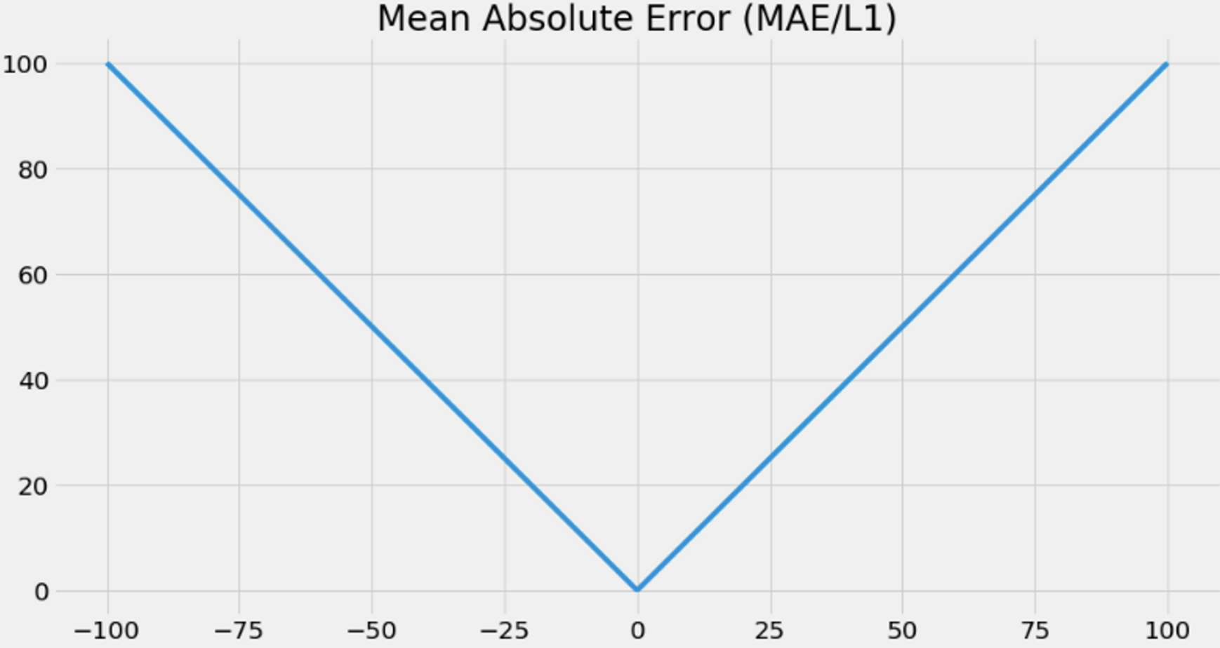
But MAE does not have its gradients decrease as the loss goes to zero. Combing MSE and MAE we have Huber loss. The Huber loss uses a hyperparameter \(\delta\) to set the threshold in which the loss goes from quadratic to linear.

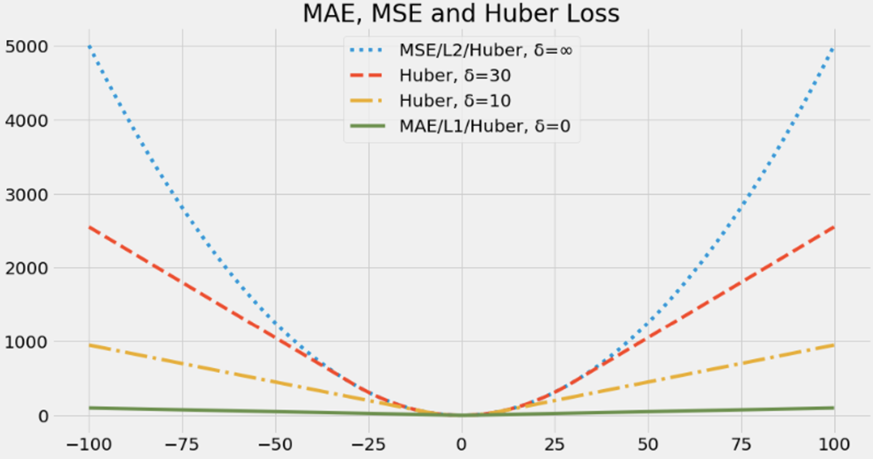
When \(\delta = 0\), it equals to MAE while when \(\delta = \infty\) it’s MSE.

The full double deep Q-network (DDQN) algorithm

Selections we made

• Approximate the action-value function \(Q(s, a; \theta)\)
• Use a state-in-values-out architecture (nodes: 4, 512, 128, 2)
• Optimize the action-value function to approximate the optimal action-value function \(q^*(s, a)\)
• Use off-policy TD targets \((r + \gamma * \max_a' Q(s', a'; \theta))\) to evaluate policies
• Use an adjustable Huber loss and set the max_gradient_norm to \(\infty\), which is MSE
• Use RMSprop as the optimizer with a learning rate of 0.0007

In DDQN, we’re still using

• An exponentially decaying epsilon-greedy strategy to improve policies, decaying from \(1.0\) to \(0.3\) in roughly \(20,000\) steps.
• Use a replay buffer with \(320\) samples min, \(50,000\) max, and mini-batches of \(64\).
• Use a target network that updates every \(15\) steps.

DDQN has three main steps:

1. Collect experiences tupes \((s, a, r, s', d)\) and insert it into the replay buffer
2. Randomly sample a mini-batch from the buffer, and calculate the off-policy TD targets \((r + \gamma * \max_{a'} Q(s', a'; \theta))\) for the whole batch
3. Fit the action-value function \(Q(s, a;\theta)\) using MSE and RMSprop