Improving Agent's Behaviors
The anatomy of reinforcement learning agents
A mental model that most reinforcement learning agents fit under.
- Reinforcement learning agent gathers experience samples, either from interacting with the environment or from querying a learned model of an environment.
- Every reinforcement learning agent learns to estimate something, perhaps a model of the environment, or possibly a policy, a value function, or just the returns.
- Every reinforcement learning agent attempts to improve a policy.
Most agents gather experience samples
One of the unique characteristics of RL is that agents learn by trial and error. The agent interacts with an environment, and as it does so, it gathers data.
Planning problems: Refers to problems in which a model of the environment is available and thus, there’s no learning required.
Learning problems: Refers to problems in which learning from samples is required, usually because there is not a model of the environment available or perhaps because it’s impossible to create one.
Most agents estimate something
After gathering data, there are multiple things an agent can do with this data.
- Certain agents, for instance, learn to predict expected returns or value functions.
- Model-based RL agents use the data collected for learning transition and reward functions.
- Moreover, agents can be designed to improve on policies directly using estimated returns.
Most agents improve a policy
Greedy policy: Refers to a policy that always selects the actions believed to yield the highest expected return from each an every state. A “greedy policy” is greedy with respect to a value function.
Epsilon-greedy policy: Refers to a policy that often selects the actions believed to yield the highest expected return from each and every state.
Optimal policy: Refers to a policy that always selects the actions actually yielding the highest expected return from each and every state. An optimal policy is a greedy policy with respect to a unique value function, the optimal value function.
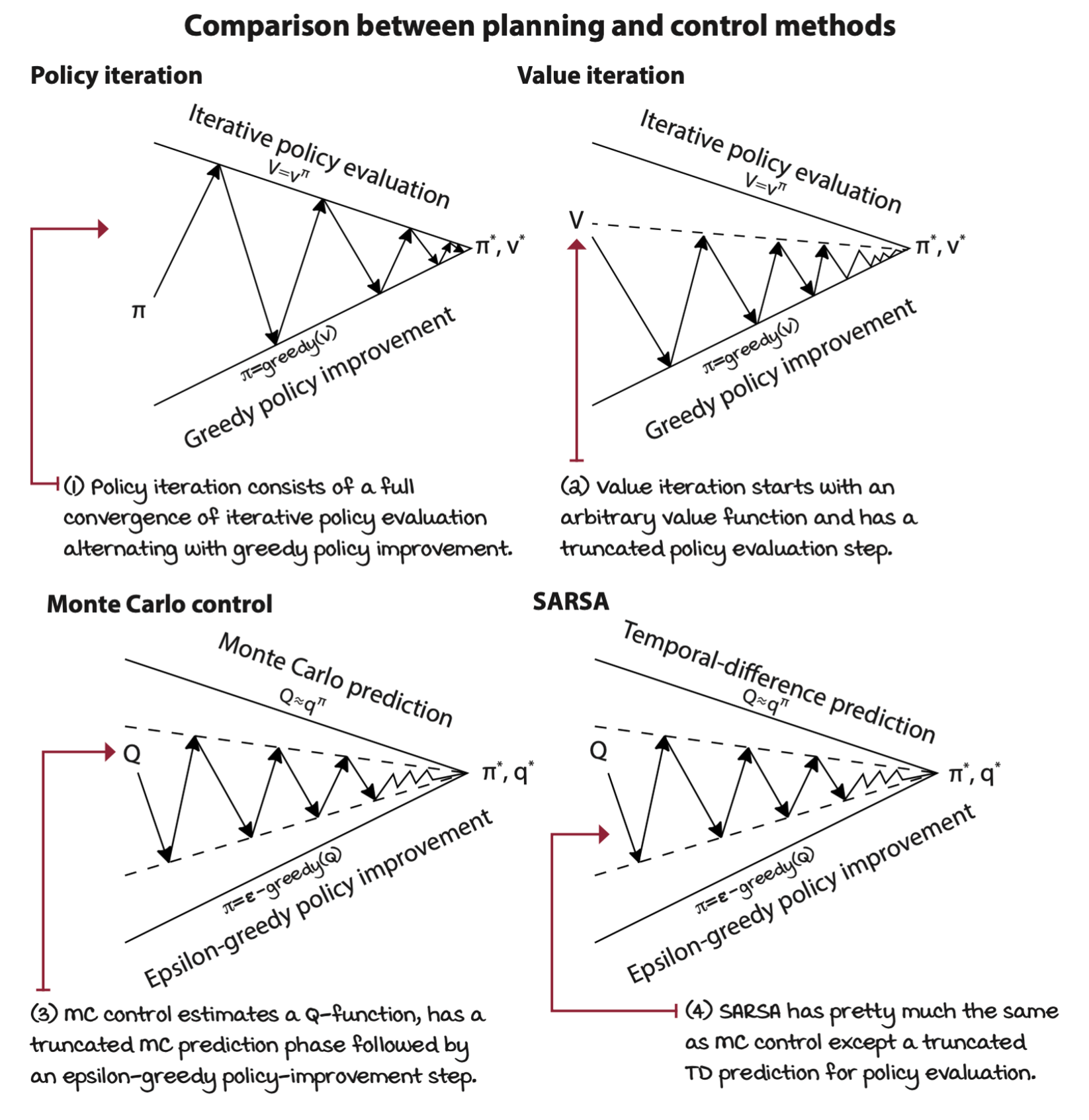
Generalized policy iteration
GPI is a general idea that the continuous interaction of policy evaluation and policy improvement drives policies towards optimality.
Learning to improve policies of behavior
Monte Carlo control: Improving policies after each episode
Let’s use first-visit Monte Carlo prediction for the policy-evaluation phase and a decaying epsilon-greedy action-selection strategy for the policy-improvement phase. But instead of rolling out several episodes for estimating the value function of a single policy using Monte Carlo prediction, we truncate the prediction step after a single full rollout and trajectory sample estimation, and improve the policy right after that single estimation step.
SARSA: Improving policies after each step
As it is discussed, one of the disadvantages of Monte Carlo methods is that they’are offline methods in an episode-to-episode sense. We must wait until we reach a terminal state before we can make improvements to our value function estimates.
By replacing MC with TD prediction, we now have a different algorithm, the well-known SARSA agent.
Decoupling behavior from learning
Q-learning: Learning to act optimally, even if we choose not to
The SARSA algorithm is a sort of “learning on the job”. The agent learns about the same policy it uses for generating experience. This type of learning is called on-policy. Off-policy learning, on the other hand, is sort of “learning from others”. The agent learns about a policy that’s different from the policy-generating experiences.
In off-policy learning, there are two policies:
- Behavior policy: used to generate experiences, to interact with the environment.
- Target policy.
The SARSA update equation is
\[ Q(S_t, A_t) \gets Q(S_t, A_t) + \alpha_t \bigg[ \overbrace{ \underbrace{ R_{t+1} + \gamma Q(S_{t+1}, A_{t+1}) }_\text{SARSA target} - Q(S_t, A_t) }^\text{SARSA error} \bigg] \]
The Q-learning’s update equation is
\[ Q(S_t, A_t) \gets Q(S_t, A_t) + \alpha_t \bigg[ \overbrace{ \underbrace{ R_{t+1} + \gamma \max_a Q(S_{t+1}, a) }_\text{Q-learning target} - Q(S_t, A_t) }^\text{Q-learning error} \bigg] \]
Q-learning uses the action with the maximum estimated value in the next state, despite the action taken.
On-policy RL algorithms, such as Monte Carlo control and SARSA, must meet the following requirements to guarantee convergence to the optimal policy:
- All state-action pairs must be explored infinitely often.
- The policy must converge on a greedy policy.
What this means in practice is that an epsilon-greedy exploration strategy, for instance, must slowly decay epsilon towards zero. If it goes down too quickly, the first condition may not be met; if it decays too slowly, well, it takes longer to converge.
But for off-policy RL algorithms, such as Q-learning, the only requirement of these two that holds is the first one.
There is another set of requirements for general convergence based on stochastic approximation theory that applies to all of these methods.
- The sum of learning rates must be infinite.
- The sum of squares of learning rates must be finite.
That means you must pick a learning rate that decays but never reaches zero. For instance, if you use 1/t or 1/e, the learning rate is initially large enough to ensure the algorithm doesn’t follow only a single sample too tightly, but becomes small enough to ensure it finds the signal behind the noise.
Double Q-learning: A max of estimates for an estimate of a max
Q-learning often overestimates the value function. On every step, we take the maximum over the estimates of the action-value function of the next state. But what we need is the actual value of the maximum action-value function of the next state.
The use of a maximum of biased estimates as the estimate of the maximum value is a problem known as maximization bias.
One way of dealing with maximization bias is to tack estimates in two Q-functions. At each time step, we choose one of them to determine the action, to determine which estimate is the highest according to that Q-function. But, then we use the other Q-function to obtain that action’s estimate. By doing this, there’s a lower chance of always having a positive bias error.