Evaluating Agent's Behaviors
In this chapter, we’ll study agents that can learn to estimate the value of policies, similar to the policy-evaluation method, but this time without the MDP. This is often called the prediction problem because we’re estimating value functions, and these are defined as the expectation of future discounted rewards.
Learning to estimate the value of policies
First-visit Monte Carlo: Improving estimates after each episode
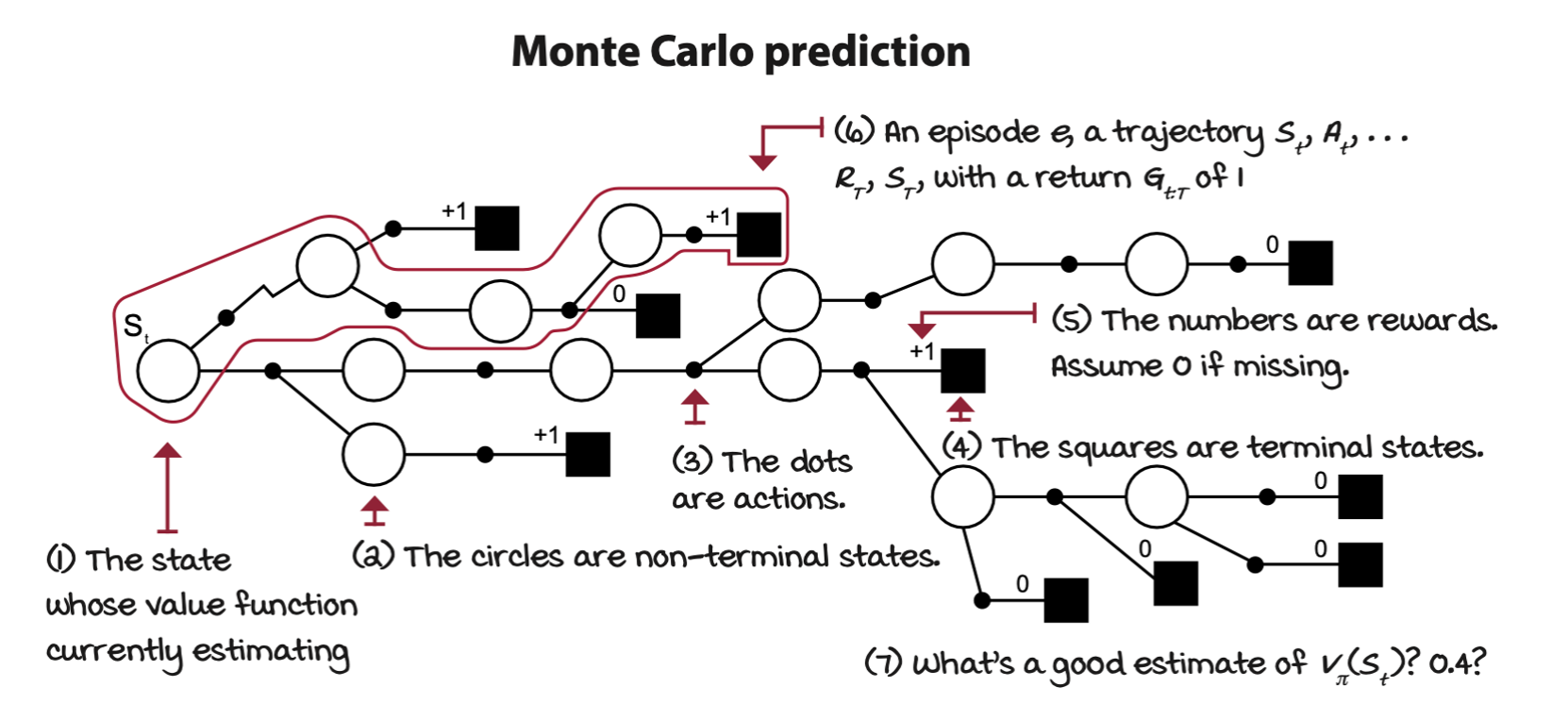
The goal is to estimate the state-value function \(v_\pi(s)\) of a policy \(\pi\). Monte Carlo prediction (MC) run episodes with a given policy and then calculate averages for every state.
The agent first interact with the environment using policy \(\pi\) util the agent hits a terminal state \(S_T\). The collection of state \(S_t\), action \(A_t\), reward \(R_{t+1}\), and next state \(S_{t+1}\) is called an experience tuple. A sequence of experiences is called a trajectory. Once a trajectory is given, returns \(G_{t:T}\) for every state \(S_t\) can be calculated. For instance, for state \(S_t\), go from time step \(t\) forward, adding up and discounting the rewards received along the way: \(R_{t+1}, R_{t+2}, R_{t+3}, \dots, R_{T}\), until the end of the trajectory at time step \(T\). Repeat the process from \(S_{t+1}\) until the final state \(S_T\), which by definition has a value of \(0\). Then discount these rewards with an exponentially decaying discount factor: \(\gamma^0, \gamma^1, \gamma^2, \dots, \gamma^{T-1}\).
After generating a trajectory and calculating the returns for all states \(S_t\), you can estimate the state-value function \(v_\pi(s)\) at the end of every episode \(e\) and final time step \(T\) by merely averaging the returns obtained from each state \(s\).
The action-value function under policy \(\pi\) is
\[ v_\pi(s) = \Bbb{E}_\pi[G_{t:T}|S_t=s] \]
and the returns are the total discounted reward
\[ G_{t:T} = R_{t+1} + \gamma R_{t+2} + \dots + \gamma^{T-1}R_T \]
Sample a trajectory from the policy
\[ S_t, A_t, R_{t+1}, S_{t+1}, \dots, R_T, S_T \sim \pi_{t:T} \]
Then add up the per-state returns and increment a count
\[ T_T(S_t) = T_T(S_t) + G_{t:T} \\ N_T(S_t) = N_T(S_t) + 1 \]
Then we can estimate the expectation using the empirial mean, so, the estimated state-value function for a state is the mean return for that state.
\[ V_T(S_t) = \frac{T_T(S_t)}{N_T(S_t)} \\ \lim_{N(s) \to \infty} V(s) = v_\pi(s) \]
Notice that means can be calculated incrementally. There is no need to keep track of the sum of returns for all states. This equation is equivalent and more efficient.
\[ V_T(S_t) = V_{T-1}(S_t) + \frac{1}{N_t(S_t)}[G_{t:T} - V_{T-1}(S_t)] \]
The mean is usually replace for a learning value that can be time dependent or constant.
\[ V_T(S_t) = V_{T-1}(S_t) + \alpha_t\bigg[ \overbrace{ \underbrace{G_{t:T}}_{\text{MC target}} - V_{T-1}(S_t) }^{\text{MC error}} \bigg] \]
Every-visit Monte Carlo: A different way of handling state visits
There are two different ways of implementing an averaging-of-returns algorithm. This is because a single trajectory may contain multiple visits to the same state. In this case, should we calculate the returns following each of those visits independently and then include all of those targets in the averages, or should we only use the first visit to each state?
Both are valid approaches, and they have similar theoretical properties. The more “standard” version is first-visit MC (FVMC), and its convergence properties are easy to justify because each trajectory is an independent and identically distributed sample of \(v_\pi(s)\). Every-visit MC (EVMC) is slightly different because returns are no longer independent and identically distributed when states are visited multiple times in the same trajectory.
Both method converge given infinite samples.
Temporal-difference learning: Improving estimates after each step
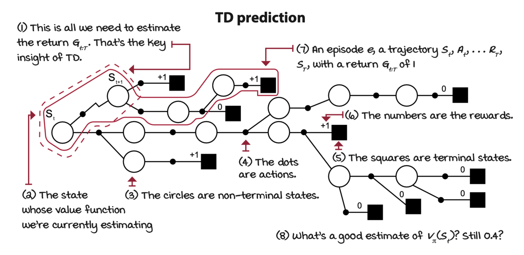
One of the main drawbacks of MC is the fact that the agent has to wait until the end of an episode when it can obtain the actual return \(G_{t:T}\) before it can update the state-value function estimate \(V_T(S_t)\). On the other hand, MC has pretty solid convergence properties because it updates the value function estimate \(V_T(S_t)\) toward the actual return \(G_{t:T}\), which is an unbiased estimate of the true state-value funtion \(v_\pi(s)\).
Also, due to the high variance of the actual returns \(G_{t:T}\), MC can be sampled inefficient. All of that randomness becomes noise that can only be alleviated with lots of data.
Instead of using the actual return \(G_{t:T}\), estimate a return. A single-step reward \(R_{t + 1}\), and once the next state \(S_{t+1}\) is observed, the state-value function estimates \(V(S_{t+1})\) can be used as an estimate of the return at the next step \(G_{t+1:T}\). This is the relationship in the equations that temporal-difference (TD) methods exploit. These methods, unlike MC, can learn from incomplete episodes by using the one-step actual return, which is the immediate reward \(R_{t+1}\), but then an estimate of the return from the next state onwards, which is the state-value function estimate of the next state \(V(S_{t+1})\), that is, \(R_{t+1} + \gamma V(S_{t+1})\), which is called the TD target.
Start from the definition of the state-value function
\[ v_\pi(s) = \Bbb{E}_\pi[G_{t:T}|S_t = s] \]
and the definition of the return in recursive form
\[ \begin{align*} G_{t:T} &= R_{t+1} + \gamma R_{t+2} + \dots + \gamma^{T-1}R_T \\ &= R_{t+1} + \gamma (R_{t+2} + \dots + \gamma^{T-2}R_T) \\ &= R_{t+1} + \gamma G_{t+1:T} \end{align*} \]
Substitute the recursive form into the state-value function
\[ \begin{align*} v_\pi(s) &= \Bbb{E}_\pi[G_{t:T}|S_t = s] \\ &= \Bbb{E}_\pi[R_{t+1} + \gamma G_{t+1:T}|S_t = s] \\ &= \Bbb{E}_\pi[R_{t+1} + \gamma \textcolor{blue}{v_\pi(S_{t+1})}|S_t = s] \end{align*} \]
Since the expectation of the returns from the next state is the state-value function of the next state, so the above definition becomes recursive. So the estimate \(V(S)\) of the true state-value function \(v_\pi(s)\) can be obtained by
\[ V_{\textcolor{blue}{t+1}}(S_t) = V_{\textcolor{blue}t}(S_t) + \alpha_t\bigg[ \overbrace{ \underbrace{R_{t+1} + \gamma V_t(S_{t+1})}_{\text{TD target}} - V_{t}(S_t) }^{\text{TD error}} \bigg] \]
A big win is we can make updates to the state-value function estimates \(V(S)\) every time step.
Learning to estimate from multiple steps
In MC methods, we sample the environment all the way through the end of the episode before we estimate the value function. On the other hand, in TD learning, the agent interacts with the environment only once, and it estimates the expected return to go to, then estimates the target then the value function. As it turns out, there’s a spectrum of algorithms lying in between MC and TD.
N-step TD learning: Improving estimates after a couple of steps
MC and TD methods can be generalized into an n-step method. Instead of doing a single step as TD or the full episode like MC, n-step TD does an n-step bootstrapping.
The experience sequence is
\[ S_t, A_t, R_{t+1}, S_{t+1}, \dots, R_{t+n}, S_{t+n} \sim \pi_{t:t+n} \]
In n-step TD we must wait n steps before we can update \(v(s)\). In MC, \(n\) is \(\infty\) while in TD, \(n\) is \(1\). The total discounted reward from step \(t\) to \(t + n\) is given by
\[ G_{t:t+n} = R_{t+1} + \dots + \gamma^{n-1} R_{t+n} + \gamma^n V_{t + n - 1}(S_{t+n}) \]
Then the state value can be estimated by
\[ V_{t+n}(S_t) = V_{t+n-1}(S_t) + \alpha\bigg[ \overbrace{ \underbrace{G_{t:t+n}}_{\text{n-step target}} - V_{t+n-1}(S_t) }^{\text{n-step error}} \bigg] \]
Forward-view TD(λ): Improving estimates of all visited states
Forward-view TD(\(\lambda\)) is a prediction method that combines multiple n-steps into a single update. In this particular version, the agent will have to wait until the end of an episode before it can update the state-value function estimates. However, another method, called, backward-view TD(\(\lambda\)), can split the corresponding updates into partial updates and apply those partial updates to the state-value function estimates on every step.
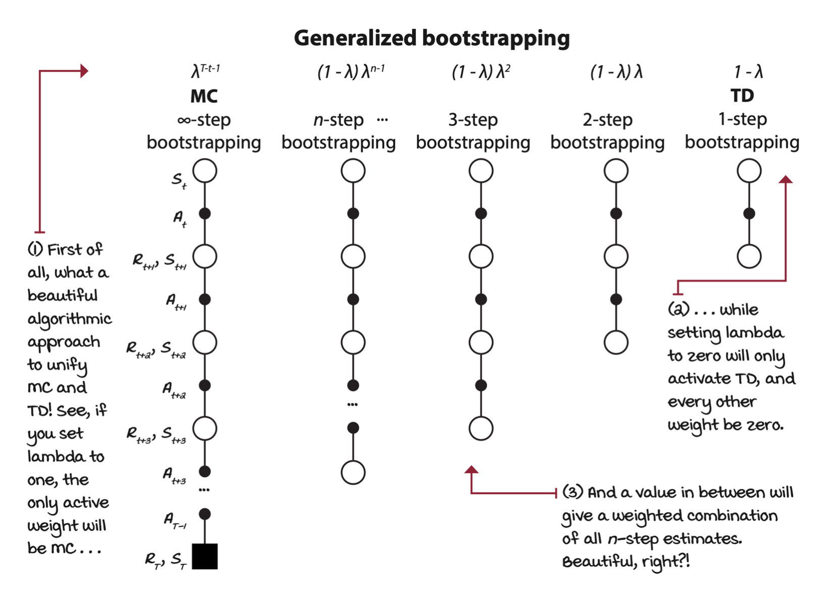
In forward view TD(\(\lambda\)), all n-step returns until the final step \(T\) are used, and weighting it with an exponentially decaying value \(\lambda\).
\[ G_{t:T}^\lambda = (1 - \lambda)\sum_{n=1}^{T-t-1} \lambda^{n-1} G_{t:t+n} + \underbrace{\lambda^{T-t-1}G_{t:T}}_\text{Weighted final return} \]
The coefficient before the weighted final return is needed so that all weights add up to 1. The above equation says that we use the following way to calculate the n-step return
\[ \begin{align*} G_{t:t+1} &= R_{t+1} + \gamma V_t(S_{t+1}) & 1 - \lambda \\ G_{t:t+2} &= R_{t+1} + \gamma R_{t+2} + \gamma^2 V_{t+1}(S_{t+2}) & (1 - \lambda)\lambda \\ G_{t:t+3} &= R_{t+1} + \gamma R_{t+2} + \gamma^2 R_{t+3} + \gamma^3 V_{t+2}(S_{t+3}) & (1 - \lambda)\lambda^2 \\ \vdots \\ G_{t:t+n} &= R_{t+1} + \cdots + \gamma^{n-1} R_{t+n} + \gamma^n V_{t+n-1}(S_{t+n}) & (1 - \lambda)\lambda^{n-1} \\ \end{align*} \]
Until the agent reaches a terminal state, then weight by this normalizing factor
\[ G_{t:T} = R_{t+1} + \gamma R_{t+2} + \dots + \gamma^{T-1} R_T \]
The final recursive equation for value state function is
\[ V_{T}(S_t) = V_{T-1}(S_t) + \alpha\bigg[ \overbrace{ \underbrace{G_{t:T}^\lambda}_{\lambda \text{-return}} - V_{T-1}(S_t) }^{\lambda \text{-error}} \bigg] \]
TD(λ): Improving estimates of all visited states after each step
MC methods are under “the curse of the time step” because they can only apply updates to the state-value function estimates after reaching a terminal state.
With n-step bootstrapping, you’re still under “the curse of the time step” because you still have to wait until \(n\) **interactions with the environment have passed before you can make an update to the state-value function estimates.
With forward-view TD(\(\lambda\)), we’re back at MC in terms of the time step.
In addition to generalizing and unifying MC and TD methods, backward-view TD(\(\lambda\)), or TD(\(\lambda\)) for short, can still tune the bias/variance trade-off in addition to the ability to apply updates on every time step.
The mechanism that provides TD(\(\lambda\)) this advantage is known as eligibility traces. An eligibility trace is a memory vector that keeps track of recently visited states. The basic idea is to track the states that are eligible for an update on every step. We keep track, not only of whether a state is eligible or not, but also by how much, so that the corresponding update is applied correctly to eligible states.
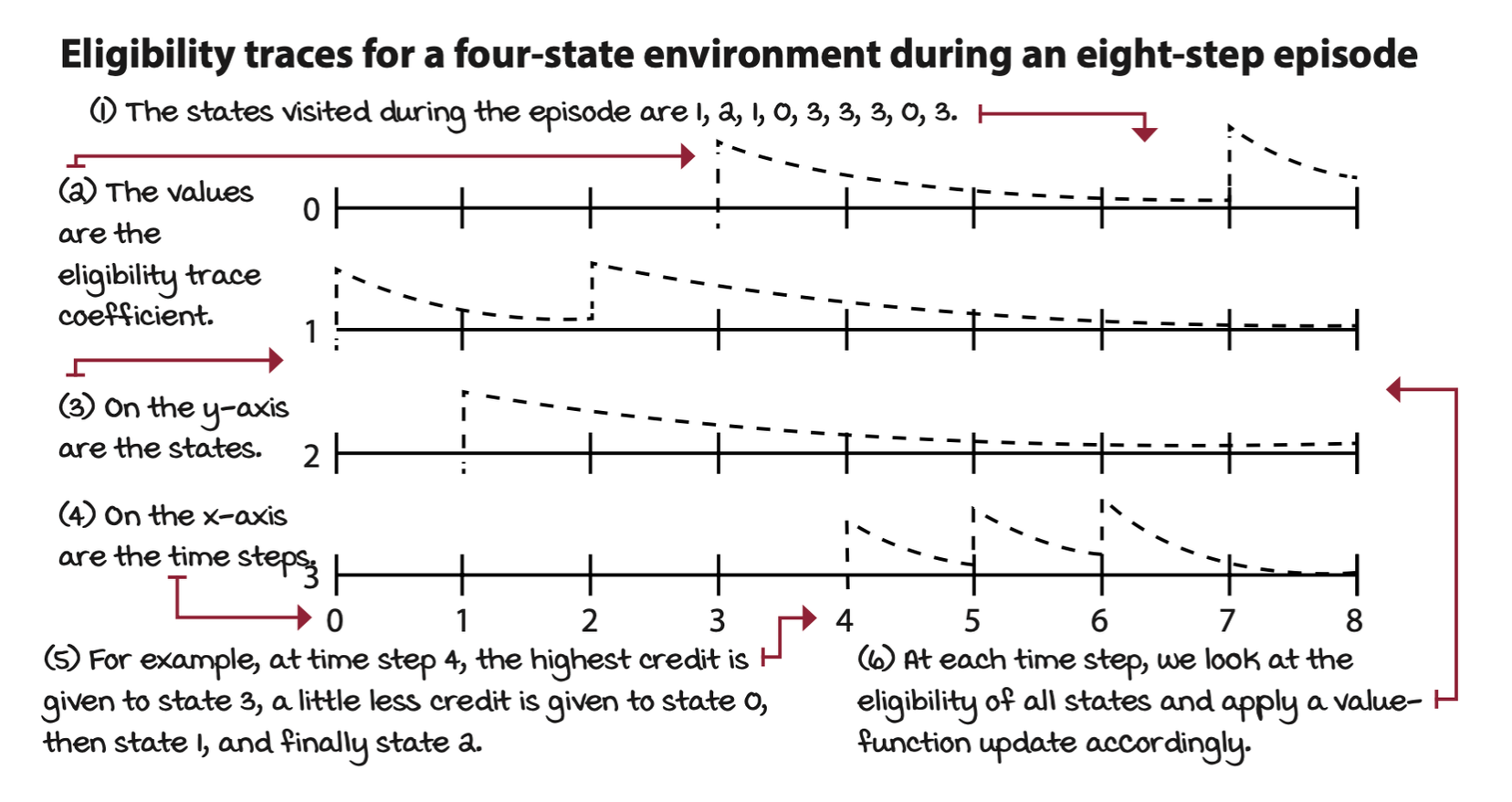
For example, all eligibility traces are initialized to zero, and when you encounter a state, you add a one to its trace. Each time step, you calculate an update to the value function for all states and multiply it by the eligibility trace vector. This way, only eligible states will get updated. After the update, the eligibility trace vector is decayed by the \(\lambda\) (weight mix-in factor) and \(\gamma\) (discount factor), so that future reinforcing events have less impact on earlier states. By doing this, the most recent states get more significant credit for a reward encountered in a recent transition than those states visited earlier in the episode, given that \(\lambda\) isn’t set to one; otherwise, this is similar to an MC update, which gives equal credit (assuming no discounting) to all states visited during the episode.
Every new episode we set the eligibility vector to \(0\).
\[ E_0 = 0 \]
Then, we interact with the environment one cycle: \(S_t, A_t, R_{t+1}, S_{t+1} \sim \pi_{t:t+1}\). Then, the eligibility of state \(S_t\) is incremented.
\[ E_t(S_t) = E_t(S_t) + 1 \]
Then calculate the TD error just as we’ve done so far
\[ \delta^\text{TD}_{t:t+1}(S_t) = \underbrace{R_{t+1} + \gamma V_t(S_{t+1})}_\text{TD target} - V_t(S_t) \]
But unlike before, we update the estimated the entire state-value function at once.
\[ V_{t+1} = V_t + \alpha_t \underbrace{\delta^\text{TD}_{t:t+1}(S_t)}_\text{TD error}E_t \]
Then we decay the eligibility
\[ E_{t+1} = E_t \gamma \lambda \]