Balancing the gathering and use of information

No matter how small and unimportant a decision may seem, every decision you make is a trade-off between information gathering and information exploitation.

The key intuition is that: exploration builds the knowledge that allows for effective exploitation, and maximum exploitation is the ultimate goal of any decision maker.

The challenge of interpreting evaluative feedback

In MAB, the Q-function of action \(a\) is

\[ q(a) = \Bbb{E}[R_t | A_t = a] \]

The best we can do in a MAB is represented by the optimal V-function, or selecting the action that maximizes the Q-function.

\[ v_* = q(a_*) = \max_{a \in A} q(a) \]

The optimal action is the action that maximize the optimal Q-function, and optimal V-function (only one state)

\[ a_* = \arg\max_{a \in A} q(a) \]

Regret: The cost of exploration

In RL, the agent needs to maximize the expected cumulative discounted reward. This means to get as much reward through the course of an episode as soon as possible despite the environment’s stochasticity. This makes sense when the environment has multiple states and the agent interacts with it for multiple time steps per episode. But in MABs, while there are multiple episodes, we only have a single chance of selecting an action in each episode.

A robust way to capture a more complete goal is for the agent to maximize the per-episode expected reward while still minimizing the total expected reward loss of rewards across all episodes. This value is called total regret, denoted by \(\tau\).

\[ \tau = \sum_{e=1}^E \Bbb{E}[v_* - q_*(A_e)] \]

which is the expectation of the difference between the optimal value of MAB and the true value of the action selected.

Approaches to solving MAB environments

The most popular and straight forward approach involves exploring by injecting randomness in our action-selection process. This family of approaches is called random exploration strategies.

Another approach to dealing with the exploration-exploitation dilemma is to be optimistic. The family of optimistic exploration strategies is a more systematic approach that quantifies the uncertainty in the decision-making problem and increases the preference for states with the highest uncertainty.

The third approach is the family of information state-space exploration strategies.

Greedy: Always exploit

Greedy strategy, or pure exploitation strategy. The greedy action selction approach consists of always selecting the action with the highest estimated value.

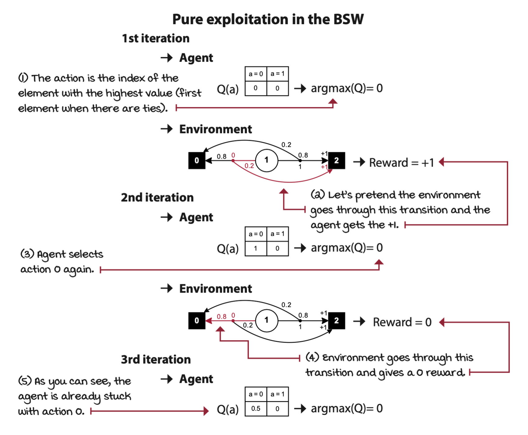
If the Q-table is initialized to zero, and there are no negative rewards in the environment, the greedy strategy will always get stuck with the first action.

💡 It is reasonable to act greedily if time is limited (one episode). Otherwise, you can’t trade-off immediate satisfaction or reward for gaining of information that would allow you better long-term results.

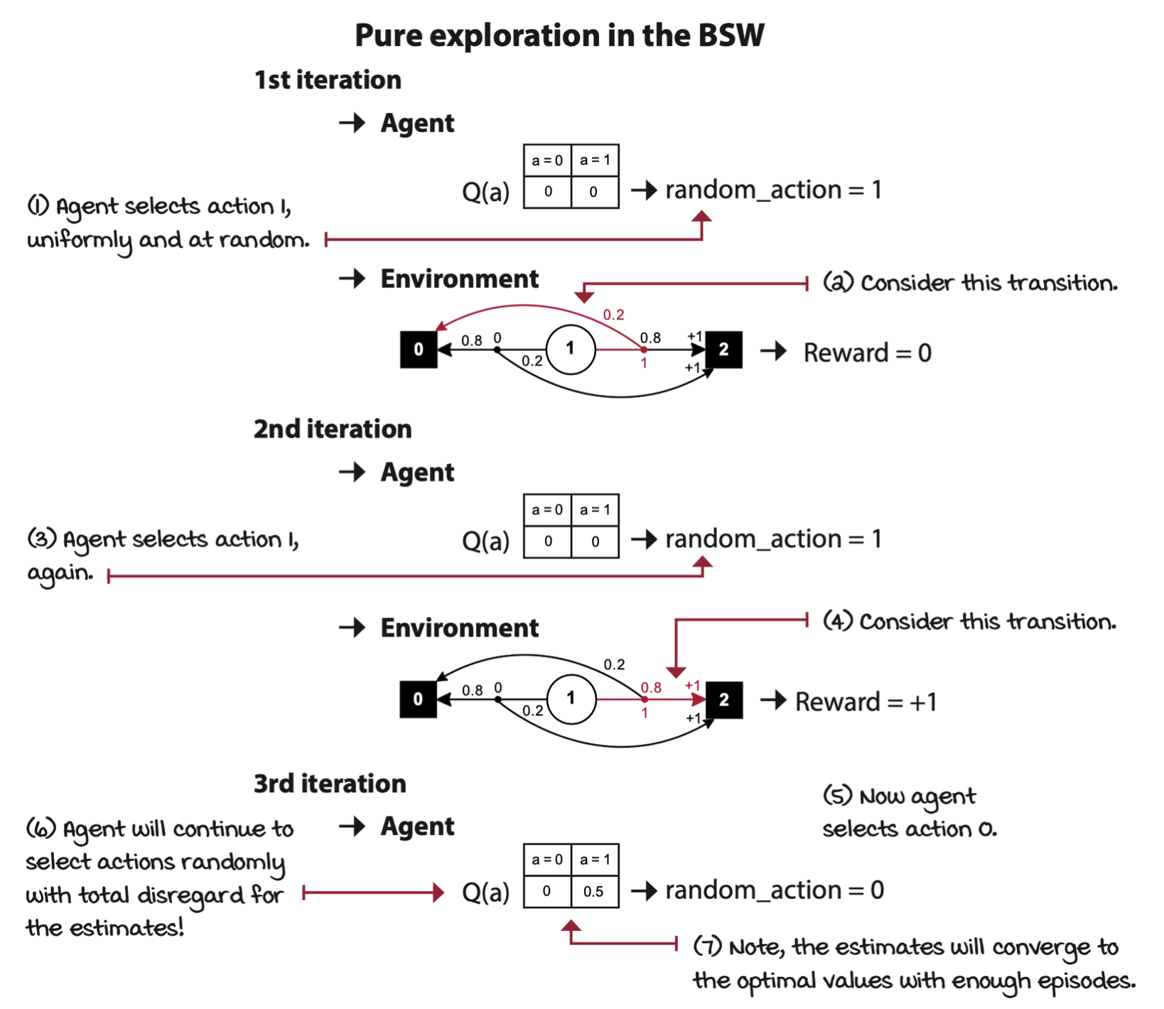
Random: Always explore

Random strategy, a pure exploration strategy. This is simply an approach to action selection with no exploitation at all.

💡 While there’s only a single way to exploit, there are multiple ways to explore. Exploiting is nothing but doing what you think is best. Exploring, on the other hand, is much more complex. It’s obvious you need to collect information. You could explore based on confidence, or based on uncertainty.

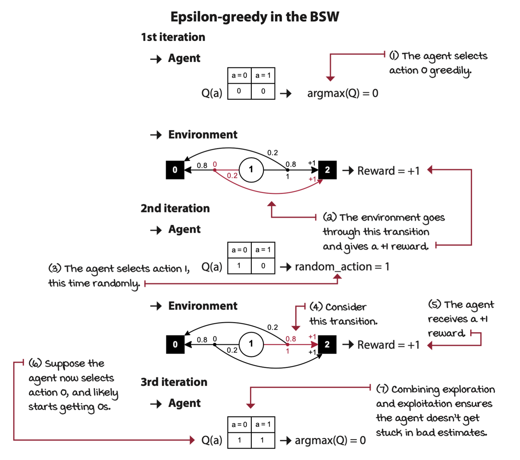
Epsilon-greedy: Almost always greedy and sometimes random

This hybrid strategy, epsilon greedy, consists of acting greedily most of the time and exploring randomly every so often. This way, the action-value function has an opportunity to converge to its true value, which in turn, will help obtain more rewards in the long term.

Decaying epsilon-greedy: First maximize exploration, then exploitation

Start with a high epsilon less than or equal to one, and decay its value on every step. This strategy, called decaying epsilon-greedy strategy.

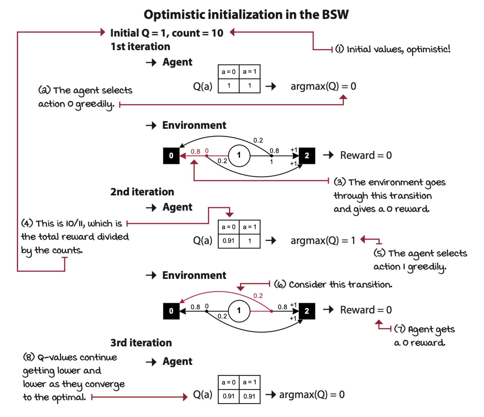
Optimistic initialization: Start off believing it’s a wonderful world

Treat actions that you haven’t sufficiently explored as if they were the best possible actions —— like you’re indeed in paradise. This class of strategies is known as optimism in the face of uncertainty. The optimistic initialization strategy is an instance of this class.

Strategic exploration

Softmax: Select actions randomly in proportion to their estimates

Random exploration strategies make more sense if they take into account Q-value estimates. Softmax strategy samples an action from a probability distribution over the action-value function such that the probability of selecting an action is proportional over the current action-value estimates.

A hyperparameter, called the temperature, can be added to control the algorithm’s sensitiviy to the differences in Q-value estimates.

The probability of selecting action \(a\) is

\[ \pi(a) = \frac{\exp\bigg[\cfrac{Q(a)}{\tau}\bigg]}{\sum^B_{b=0} \exp\bigg[\cfrac{Q(b)}{\tau}\bigg]} \]

where \(\tau\) is the temperature parameter.

UCB: It’s not about optimism, it’s about realistic optimism

There are two inconveniences with the optimistic initialization algorithm:

1. We don’t always know the maximum reward the agent can obtain from an environment. If the initial Q-value is set to be much higher than the actual maximum value, then the algorithm will perform sub-optimally because the agent will take many episodes to bring the estimates near the actual values. But even worse, if the Q-values are set to a value lower than the environment’s maximum, the algorithm will no longer be optimistic.
2. The “counts” variable in the optimistic initialization is a hyperparameter and it needs tuning, but in reality, what we’re trying to represent with this variable is the uncertainty of the estimate, which shouldn’t be a hyperparameter.

Upper confidence bound (UCB) strategy solve the problem. In UCB, instead of blindly hoping for the best, we look at the uncertainty of value estimates. The more uncertain a Q-value estimate, the more critical it is to explore it.

\[ A_e = \arg\max_a \bigg[ Q_e(a) + c \sqrt{\frac{\ln e}{N_e(a)}}\bigg] \]

To implement the strategy, we select the action with the highest sum of its Q-value estimate and an action-uncertainty bonus \(U\). If we attempt action \(a\) only a few times, the \(U\) bonus is large, thus encouraging exploring this action. Otherwise, we only add a small \(U\) bonus value to the Q-value estimates.

Thompson sampling: Balancing reward and risk

Thompson sampling strategy is a sample-based probability matching strategy that allows us to use Bayesian techniques to balance the exploration and exploitation trade-off.

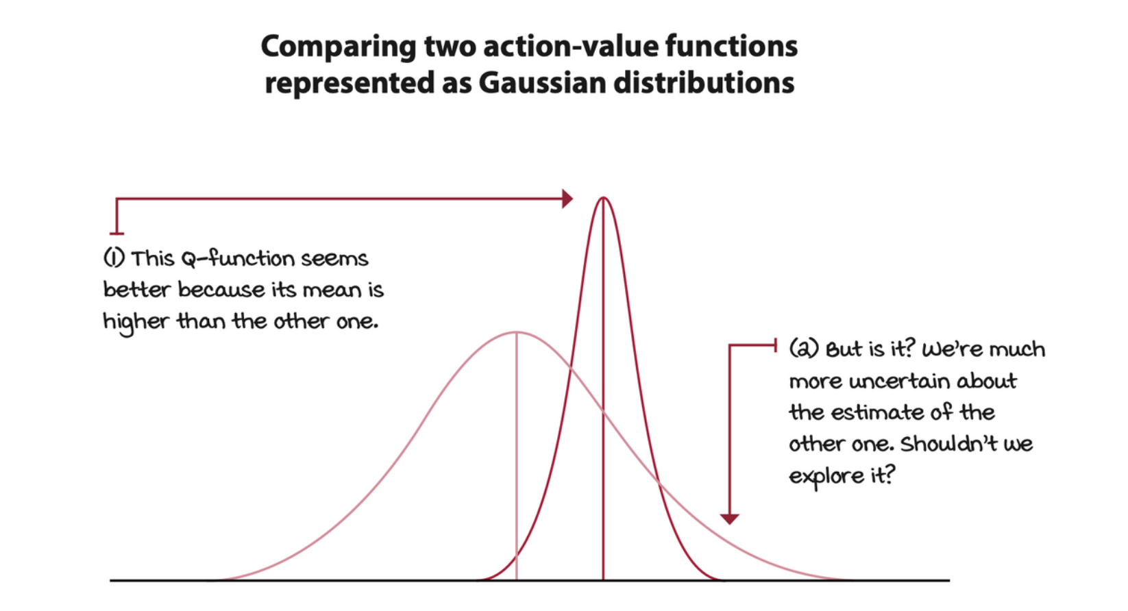
As the name suggests, in Thompson sampling, we sample from these normal distributions and pick the action that returns the highest sample. Then, to update the Gaussian distributions’ standard deviation, we use a formula similar to the UCB strategy in which, early on when the uncertainty is higher, the standard deviation is more significant; therefore, the Gaussian is broad. But as the episodes progress, and the means shift toward better and better estimates, the standard deviations gets lower, and the Gaussian distribution shrinks, and so its samples are more and more likely to be near the estimated mean.