Balancing immediate and long-term goals
The objective of a decision-making agent
At first, it seems the agent’s goal is to find a sequence of actions that will maximize the return: the sum of rewards during an episode or the entire life of the agent. But, plans are not enough in stochastic environments. What the agent needs to come up with is called policy.
Policies are universal plans, they cover all possible states.
Policies: Per-state action prescriptions
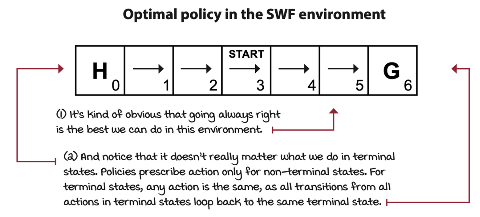
Given the environment, the agent needs to find a policy, denoted as \(\pi\). A policy is a function that prescribes actions to take for a given nonterminal state.
State-value function: What to expect from here?
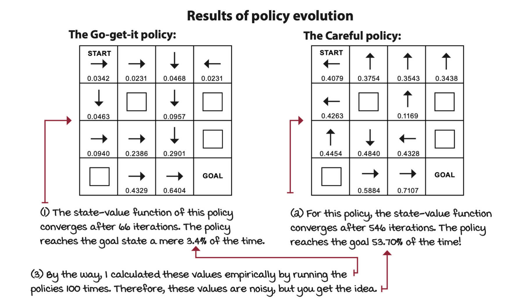
If a policy and the MDP is given, we would be able to calculate the expected return starting from every single state. The value of a state \(s\) under policy \(\pi\) is the expectation of returns if the agent follows policy \(\pi\) starting from state \(s\). Calculate this for every state, and you get the state-value function, or V-function.
\[ \begin{align*} \blue{v_\pi(s)} &= \Bbb{E}_\pi [G_t | S_t = s] \\ &= \Bbb{E}_\pi [R_{t+1} + \gamma R_{t+2} + \gamma^2 R_{t+3} + \dots | S_t = s] \\ &= \Bbb{E}_\pi [R_{t+1} + \gamma G_{t+1} | S_t = s] \\ &= \sum_a \pi(a|s) \sum_{s', r} p(s', r|s, a)[r + \gamma \blue{v_\pi(s')}], \forall s \in S \end{align*} \]
The above function is call Bellman equation. Note that the equation is given in recursive form.
Action-value function: What should I expect from here if I do this?
Another critical question that we often need to ask is the value of taking action \(a\) in a state \(s\). The action-value function, also known as Q-function or \(Q_\pi (s, a)\), captures the expected return if the agent follows policy \(\pi\) after taking action \(a\) in state \(s\).
\[ \begin{align*} q_\pi(s, a) &= \Bbb{E}_\pi[G_t | S_t = s, A_t = a] \\ &= \Bbb{E}_\pi[R_t + \gamma G_{t+1} | S_t = s, A_t = a] \\ &= \sum_{s', r} p(s', r|s, a)[r + \gamma v_\pi(s')], \forall s \in S, \forall a \in A \end{align*} \]
The above function is the Bellman equation for action values.
Action-advantage function: How much better if I do that?
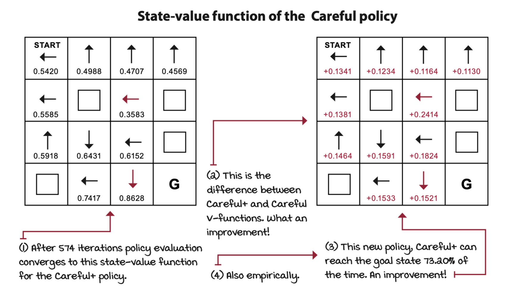
The advantage function, also known as the A-function, or \(A_\pi(s, a)\), is the difference between the action-value function of action \(a\) in state \(s\) and the state-value function of state \(s\) under policy \(\pi\).
\[ a_\pi(s, a) = q_\pi(s, a) - v_\pi(s) \]
The advantage function describes how much better it is to take action \(a\) instead of following policy \(\pi\).
Optimality
Policies, state-value functions, action-value functions, and action-advantage functions are the components we use to describe, evaluate, and improve behaviors. We call it optimality when these components are the best they can be.
An optimal policy is a policy that for every state can obtain expected returns greater than or equal to any other policy.
\[ \begin{align*} v_*(s) &= \max_\pi v_\pi(s), \forall s \in S \\ q_*(s, a) &= \max_\pi q_\pi(s, a), \forall s \in S, \forall a \in A(s) \\ v_*(s) &= \max_a \sum_{s', r} p(s', r|s, a)[r + \gamma v_*(s')] \\ q_*(s, a) &= \sum_{s', r} p(s', r|s, a)[r + \gamma \max_a' q_*(s', a')] \end{align*} \]
Planning optimal sequences of actions
Policy evaluation: Rating policies
The policy-evaluation algorithm consists of calculating the V-function for a given policy by sweeping through the state space and iteratively improving estimates.
Policy-evaluation equation
The policy-evaluation algorithm consist of the iterative approximation of the state-value function of the policy under evaluation. The algorithm converges as \(k\) approaches infinity.
Initialize \(v_0(s)\) for all \(s\) in \(S\) arbitrarily, and to \(0\) is \(s\) is terminal. Then, increase \(k\) and iteratively improve the estimates by following the equation below.
\[ v_{k+1}(s) = \sum_a \pi(a|s) \sum_{s', r} p(s', r|s, a)[r + \gamma v_k(s')] \]
def policy_evaluation(pi, P, gamma=1.0, theta=1e-10): |
Policy improvement: Using ratings to get better
Using the V-function and the MDP, you get an estimate of the Q-function. The Q-function will give you a glimpse of the values of all actions for all states, and these values, can hint at how to improve policies.
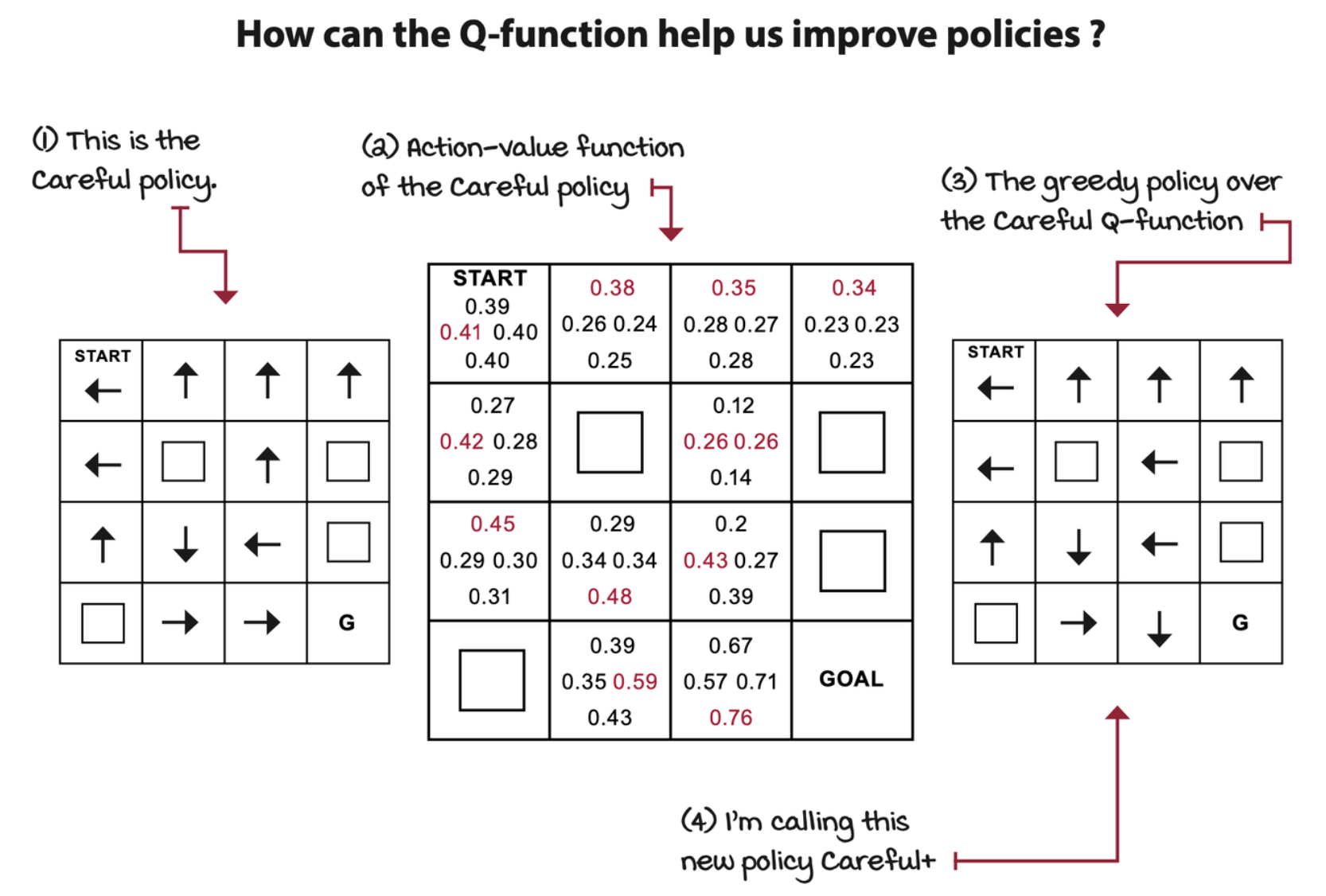
We used the state-value function of the original policy and the MDP to calculate its action-value function. Then, acting greedily with respect to the action-value function gave us an improved policy.
\[ \pi'(s) = \argmax_a \sum_{s', r} p(s', r|s, a)[r + \gamma v_\pi(s')] \]
New policy \(\pi'\) is obtained by taking the highest-valued action. The valued action is calculated by the weighted sum of all rewards and values of all possible next states.
def policy_improvement(V, P, gamma=1.0): |
Policy iteration (PI)
Policy iteration algorithm starts with random policy, then use the V-function and Q-function to improve the policy.
def policy_iteration(P, gamma=1.0, theta=1e-10): |
The policy iteration is guaranteed to converge to the exact optimal policy: the mathematical proof shows it will not get stuck in local optima.
Value iteration (VI): Improving behaviors early
VI can be thought of “greedily greedifying policies” because we calculate the greedy policy as soon as we can, greedily. VI doesn’t wait until we have an accurate estimate of the policy before it improves it, but instead, VI truncates the policy-evaluation phase after a single state sweep.
We can merge a truncated policy-evaluation step and a policy improvement into the same equation.
\[ v_{k+1}(s) = \max_a \sum_{s', r} p(s', r|s, a)[r + \gamma v_k(s')] \]
In VI, we don’t have to deal with policies at all. While the goal of VI is the same as the goal of PI —— to find the optimal policy for a given MDP —— VI happens to do this through the value functions.
Whereas VI and PI are two different algorithms, in a more general view, they are two instances of generalized policy iteration (GPI). GPI is a general idea in RL in which policies are improved using their value function estimates, and value function estimates are improved toward the actual value function for the current policy.
def value_iteration(P, gamma=1.0, theta=1e-10): |