Mathematical foundations of reinforcement learning
Complex sequential decision-making under uncertainty.
- Complex: the agents may be learning in environments with vast state and action spaces.
- Sequantial: in many problems, there are delayed consequences.
- Uncertainty: we don’t know the actual inner workings of the world to understand how our actions affect it.
A mathematical framework known as Markov decision processes (MDPs) is used to represent these kinds of problems. The general framework of MDPs allows us to model virtually any complex sequential decision-making problem under uncertainty in a way that RL agents can interact with and learn to solve solely through experience.
Components of reinforcement learning
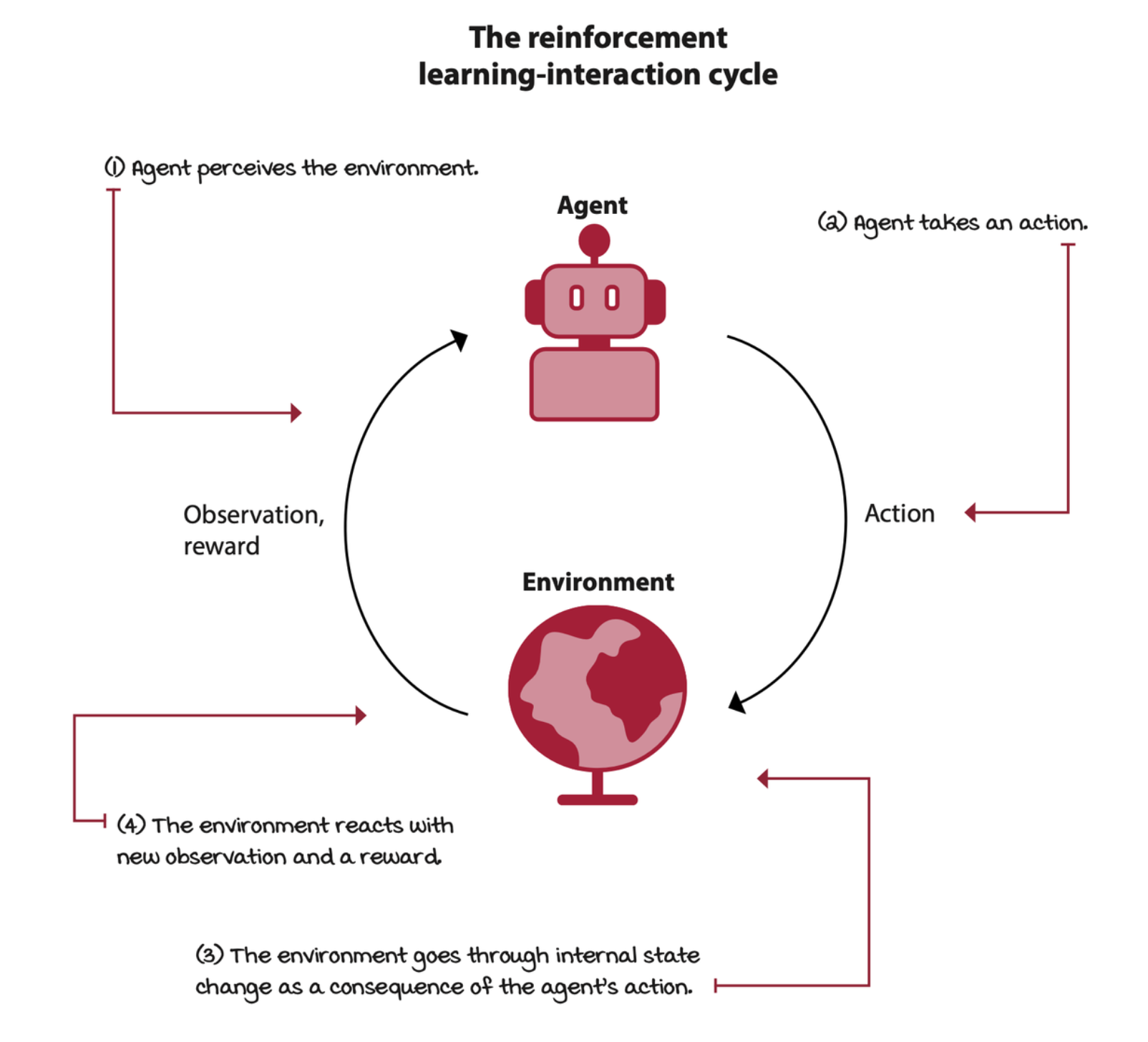
The two core components in RL are the agent and the environment. The agetn is the decision maker, and is the solution to a problem. The environment is the representation of a problem.
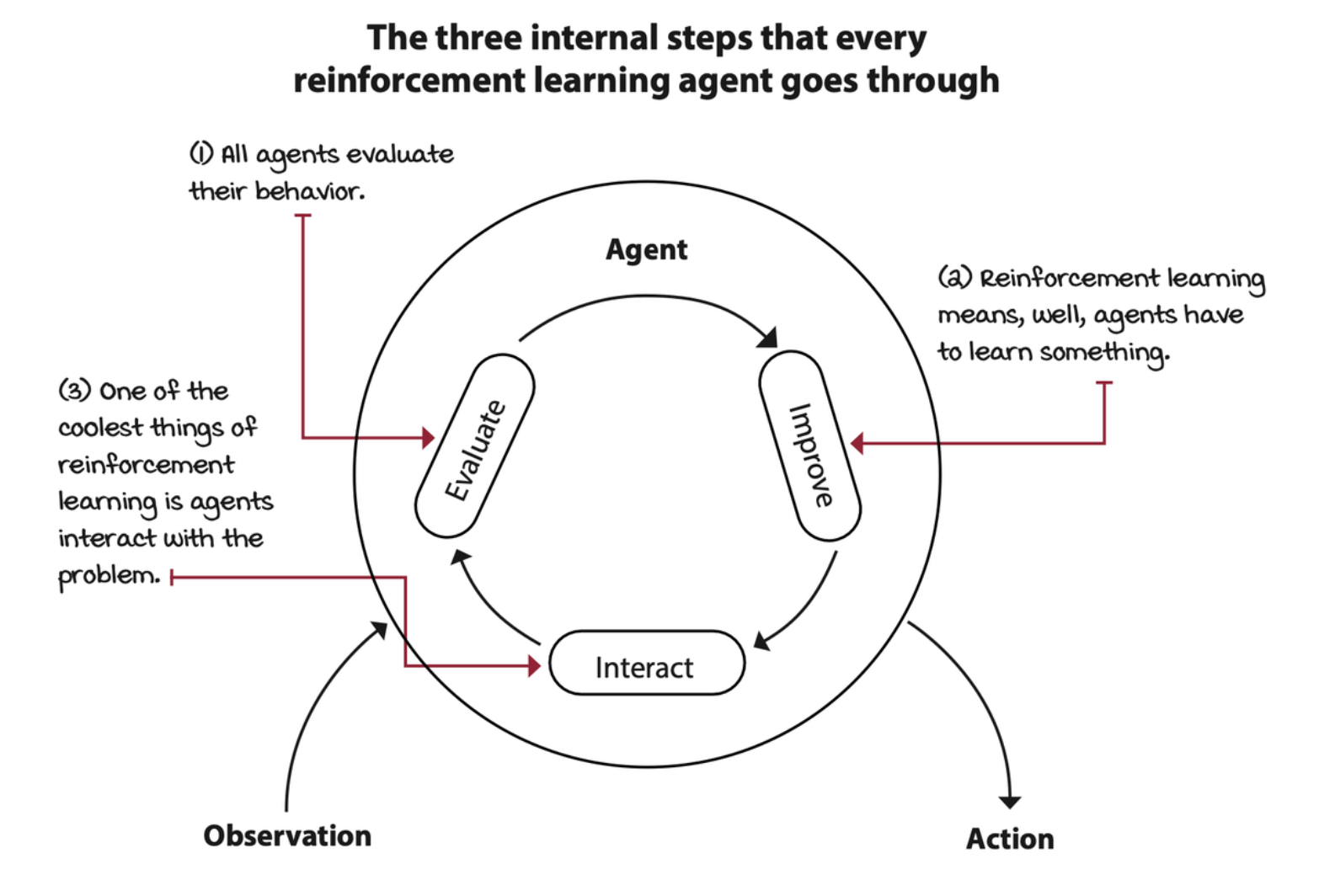
The agent: The decision maker
Most agents have a three-step process:
- Interaction: a way to gather data for learning
- Evaluate: current behavior
- Improve: inner components that allows them to improve their overall performance
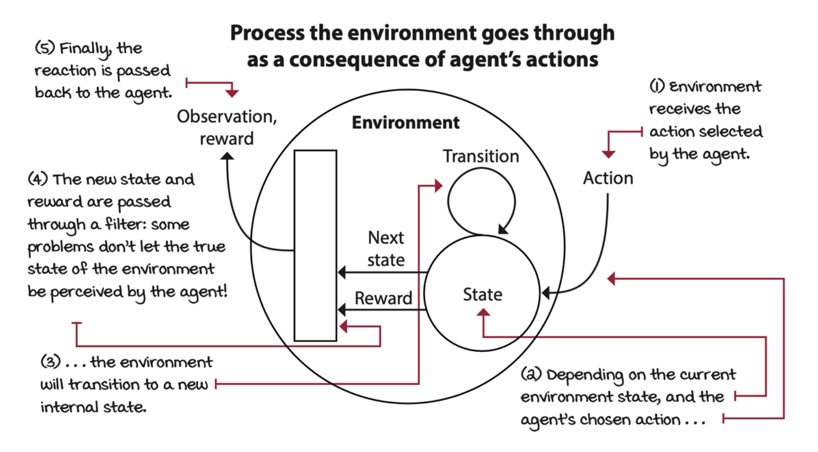
The environment: everything else
Most real-world decision-making problems can be expressed as RL environments. A common way to represent decision-making processes in RL is by modeling the problem using a mathematical framework known as Markov decision processes (MDPs). In RL, we assume all environments have an MDP working under the hood.
The environment is represented by a set of variables related to the problem. The combination of all the possible values this set of variables can take is referred to as the state space. A state is a specific set of values the variables take at any given time.
The set of variables the agent perceives at any given time is called an observation. The combination of all possible values these variables can take is the observation space.
At every state, the environment makes available a set of actions the agent can choose from. The set of all actions in all states is referred to as the action space.
The agent attempts to influence the environment through these actions. The environment may change states as a response to the agent’s action. The function that is responsible for this transition is called the transition function.
After a transition, the environment emits a new observation. The environment may also provide a reward signal as a response. The function responsible for this mapping is called the reward function. The set of transition and reward function is referred to as the model **of the environment.
Agent-environment interaction cycle
To represent the ability to interact with an environment in an MDP, we need states, observations, actions, a transition, and a reward function.
The interactions between the agent and the environment go on for several cycles. Each cycle is called a time step. The set of the observation (or state), the action, the reward, and the new observation (or new state) is called an experience tuple.
MDPs: The engine of the environment
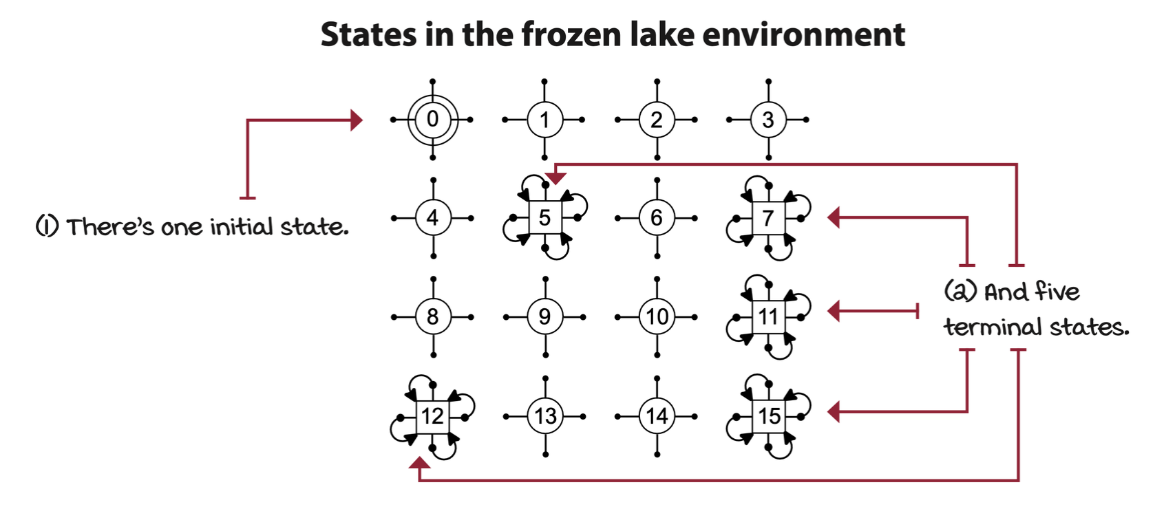
States: Specific configuarations of the environment
A state is a unique and self-contained configuration of the problem. The set of all possible states, the state space, is defined as the set \(S\).
The probability of the next state, given the current state and action, is independent of the history of interactions. This memoryless property of MDPs is known as the Markov property.
\[ P(S_{t + 1} | S_t, A_t) = P(S_{t+1}|S_t, A_t, S_{t-1}, A_{t-1}, \dots) \]
The set of all states in the MDP is denoted \(S^+\). The set of starting or initial states, denoted \(S^i\). The set of all non-terminal states is denoted \(S\).
Actions: A mechanism to influence the environment
MDPs make available a set of actions \(A\) that depends on the state. In fact, \(A\) is a function that takes a state as an argument, that is, \(A(s)\). This function returns a set of available actions for state \(s\).
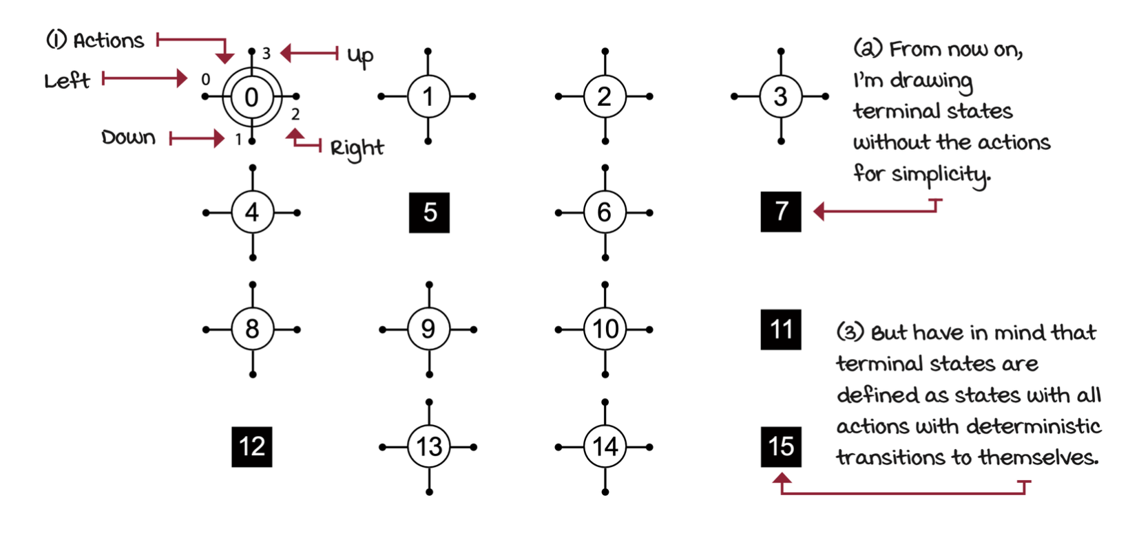
For generalization, terminal states are defined as states with all actions with deterministic transitions to themselves.
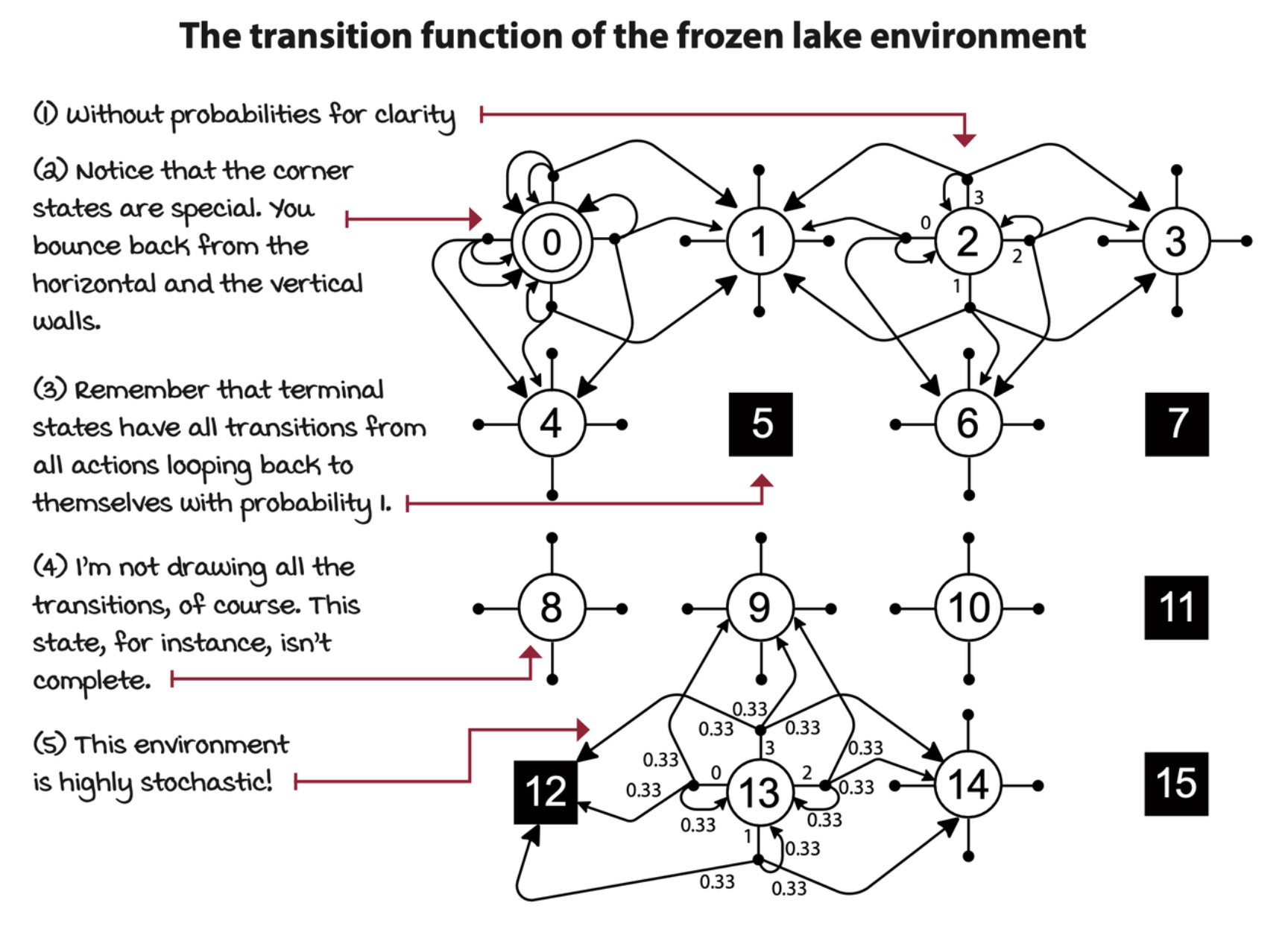
Transition function: Consequences of agent actions
The way the environment changes as a response to actions is referred to as the state-trainsition probabilities, or, the transition function, and is denoted by \(T(s, a, s')\). The transition function \(T\) maps \(s, a, s'\) to a probability. It can also be represented as \(T(s, a)\) and return a dictionary with the next states for its keys and probabilities for its values.
The transition function is defined as
\[ p(s'|s, a) = P(S_t = s'|S_{t - 1} = s, A_{t - 1} = a) \\ \sum_{s' \in S} p(s'|s, a) = 1, \forall s \in S, \forall a \in A(s) \]
One key assumption of many RL (and DRL) algorithms is that this distribution is stationary.
Reward signal
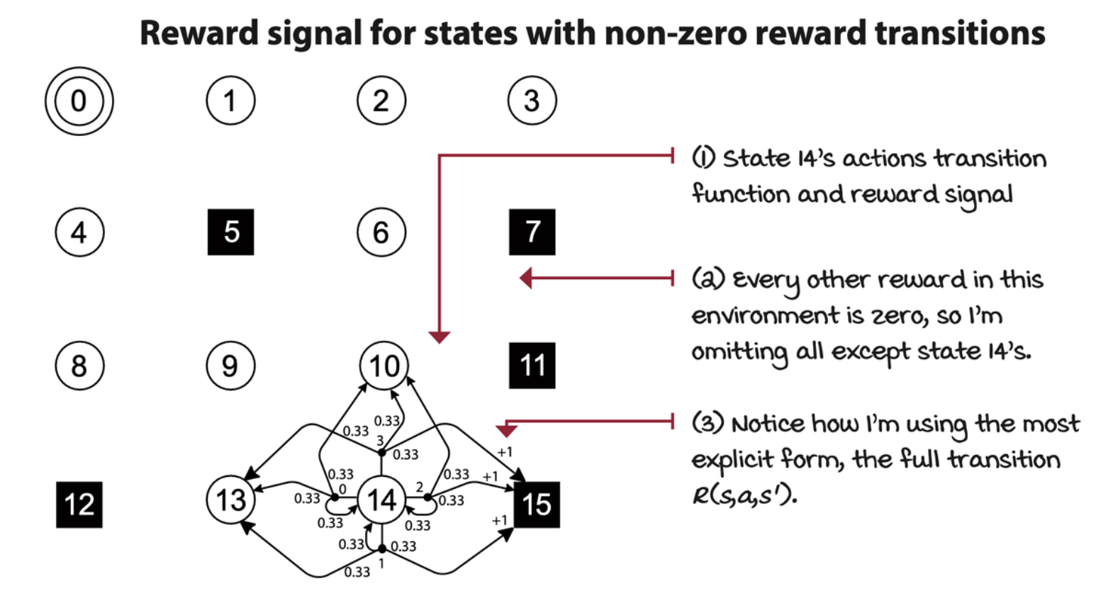
The reward function \(R\) maps a transition tuple \(s, a, s'\) to a scalar. The reward function gives a numeric signal of goodness to transitions. With that, we can compute the marginalization over next states in \(R(s,a,s')\) to obtain \(R(s,a)\), and the marginalization over actions in \(R(s,a)\) to get \(R(s)\).
\[ r(s,a,s') = \Bbb E[R_t | S_{t-1} = s, A_{t-1} = a, S_t = s'] \\ R_t \in R \sub \R \]
The reward of \(s, a, s'\) tuple is the expectation of reward at time step \(t\) given the tuple. The reward at time step \(t\) comes from a set of all rewards \(R\), which is a subset of all real numbers.
Horizon: Time changes what’s optimal
We can represent time in MDPs as well. A time step is a global clock syncing all parties and discretizing time. An episodic task is a task in which there’s a finite number of time steps, either because the clock stops or because the agent reaches a terminal state. There are also continuing tasks, which are tasks that go on forever.
Episodic and continuing tasks can also be defined from the agent’s perspective. It is called planning horizon. On the other hand, a finite horizon is a planning horizon in which the agent knows that task will terminate in a finite number of time steps. On the other hand, an infinite horizon is when the agent doesn’t have a predetermined time step limit, so the agent plans for an infinite number of time steps.
Discount: The future is uncertain, value it less
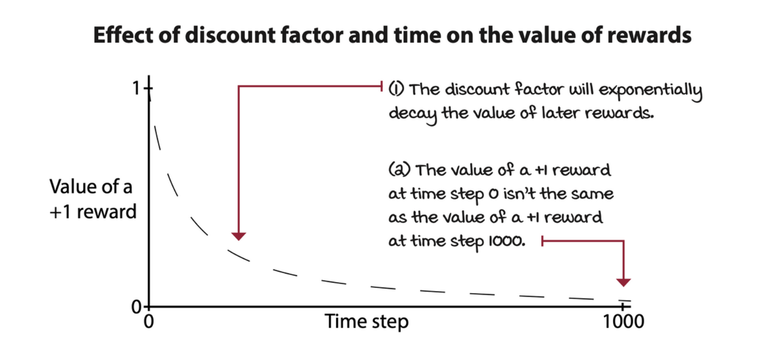
Because of the possibility of infinite sequences of time steps in infinite horizon tasks, we need a way to discount the value of rewards over time. It is common to use a positive real value less than one to exponentially discount the value of future rewards.
This number is called the discount factor, or gamma.
💡 Interestingly, gamma is part of the MDP definition: the problem, and not the agent.
The sum of all rewards obtained during the course of an episode is referred to as the return.
\[ G_t = R_{t+1} + R_{t+2} + \cdots + R_T \]
The discount factor is used to downweight rewards that occur later during the episode.
\[ \begin{align*} G_t &= R_{t+ 1} + \gamma R_{t+2} + \gamma^2 R_{t+3} + \cdots + \gamma^{T-1} R_T \\ &= \sum_{k=0}^\infty \gamma^k R_{t+k+1} \end{align*} \]
It can also be represented by recursive definition.
\[ G_t = R_{t+1} + \gamma G_{t+1} \]
💡 MDPs vs. POMDPs
\(\textbf{MDP}(S, A, T, R, S_\theta, \gamma, H)\) have state space \(S\), action space \(A\), transition function \(T\), reward signal \(R\). They also has a set of initial states distribution \(S_\theta\), the discount factor \(\gamma\), and the horizon \(H\).
\(\textbf{POMDP}(S, A, T, R, S_\theta, \gamma, H, O, \varepsilon)\) adds the observation space \(O\) and an emission probability \(\varepsilon\) that defines the probability of showing an observation \(o_t\) given a state \(s_t\).