Quantifying Uncertainty

Acting under Uncertainty

The rational decision —— depends on both the relative importance of various goals and the likelihood that, and degree to which, they will be achieved.

Summarizing Uncertainty

Uncertainty and Rational Decisions

An agent must have preferences among the different possible outcomes of the various plans. An outcome is a completely specified state. We use utility theory to represent preferences and reason quantitatively with them.

Preferences, as expressed by utilities, are combined with probabilities in the general theory of rational decisions called decision theory:

\[ \text{decision theory} = \text{probability theory} + \text{utility theory} \]

The fundamental idea of decision theory is that an agent is rational if and only if it chooses the action that yields the highest expected utility, averaged over all the possible outcomes of the action. This is called the principle of maximum expected utility (MEU).

// A decision-theoretic agent
function DT_Agent(percept: Percept): Action {
    // probabilistic beliefs about the current state of the world
    const beliefState
    // the agent's action
    const action

    beliefState.update(action, percept)
    const probabilities = CalculateProbabilities(
        ActionDescriptions,
        beliefState.current
    )
    action = SelectAction(
        probabilities,
        utilityInformation
    )

    return action
}

Basic Probability Notation

Probabilities

The set of all possible worlds is called the sample space. The possible worlds are mutually exclusive and exhaustive. \(\Omega\) is used to refer to the sample space, and \(\omega\) refers to elements of the space.

A fully specified probability model associates a numerical probability \(P(\omega)\) with each possible world.

\[ 0 \leq P(\omega) \leq 1 \text{ for every } \omega \text{ and } \sum_{\omega \in \Omega} P(\omega) = 1 \]

Probabilistic assertions and queries are not usually about particular possible worlds, but about sets of them. In probability theory, these sets are called events. In logic, a set of worlds corresponds to a proposition in a formal language. The probability associated with a proposition is defined to be the sum of the probabilities of the worlds in which it holds

\[ \text{For any proposition } \phi, P(\phi) = \sum_{\omega \in \phi} P(\omega) \]

Unconditional probabilities are called prior probabilities, they refer to degrees of belief in propositions in the absence of any other information. Conditional probabilities are called posterior probabilities, which is defined as

\[ P(a|b) = \frac{P(a \land b)}{P(b)} \]

The Language of Propositions in Probability Assertions

Variables in probability theory are called random variables. Every random variable is a function that maps from the domain of possible worlds \(\Omega\) to some range —— the set of possible values it can take on.

Variables can have infinitive ranges, either discrete or continuous.

For example, “the probability that the patient has a cavity, given that she is a teenager with no toothache, is 0.1” can be expressed as follows:

\[ P(cavity | \lnot toothache \land teen) = 0.1 \]

Probability Axioms and their Reasonableness

The formula for the probability of a disjunction, sometimes called the inclusion-exclusion principle.

\[ P(a \lor b) = P(a) + P(b) - P(a \land b) \]

De Finettis’ theorem is not concerned with choosing the right values for individual probabilities, but with choosing values for the probabilities of logically related propositions.

Inference Using Full Joint Distributions

Probabilistic inference, the computation of posterior probabilities for query propositions given observed evidence. The full joint distribution is used as a knowledge base from which answers to all questions may be derived.

Marginalization rule:

\[ \textbf{P}(\textbf{Y}) = \sum_\textbf{Z}\textbf{P}(\textbf{Y}, \textbf{Z} = \textbf{z}) \]

where \(\sum_{\textbf{Z}}\) sums over all the possible combinations of values of the set of variables \(\textbf{Z}\). Using the product rule, obtaining a rule called conditioning.

\[ \textbf{P}(\textbf{Y}) = \sum_\textbf{Z} \textbf{P}(\textbf{Y}|\textbf{z})P(\textbf{z}) \]

General inference procedure. Let the query involve only a single variable, \(X\). Let \(\textbf{E}\) be the list of evidence variables. Let \(\textbf{e}\) be the list of observed values for them, and let \(\textbf{Y}\) be the remaining unobserved variables. The query is \(\textbf{P}(X | \textbf{e})\) and can be evaluated as

\[ \textbf{P}(X | \textbf{e}) = \alpha \textbf{P}(X, \textbf{e}) = \alpha \sum_\textbf{y} \textbf{P}(X, \textbf{e}, \textbf{y}) \]

💡 The full joint distribution in tabular form is seldom a practical tool for building reasoning systems. Instead, it should be viewed as the theoretical foundation on which more effective approaches may be built, just as truth tables formed a theoretical foundation for more practical algorithms like DPLL.

Independence

Independence between propositions \(a\) and \(b\) can be written as

\[ P(a|b) = P(a) \text{ or } P(b|a) = P(b) \text{ or } P(a\land b) = P(a)P(b) \]

Two examples of factoring a large joint distribution into smaller distributions, using absolute independence. (a) Weather and dental problems are independent. (b) Coin flips are independent.

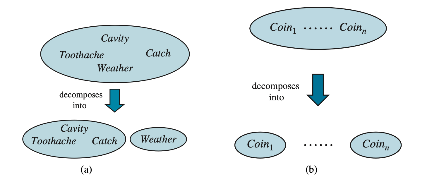
Two examples of factoring a large joint distribution into smaller distributions, using absolute independence. (a) Weather and dental problems are independent. (b) Coin flips are independent.

Bayes’ Rule and Its Use

Basic version of Bayes’ rule.

\[ P(b|a) = \frac{P(a|b)P(b)}{P(a)} \]

A more general version of Bayes’ rule.

\[ \textbf{P}(Y|X) = \frac{\textbf{P}(X|Y)\textbf{P}(Y)}{\textbf{P}(X)} \]

A more general version conditionalized on some background evidence \(\textbf{e}\).

\[ \textbf{P}(Y|X, \textbf{e}) = \frac{\textbf{P}(X|Y, \textbf{e})\textbf{P}(Y|\textbf{e})}{\textbf{P}(X|\textbf{e})} \]

Applying Bayes’ Rule: The Simple Case

Often, we perceive as evidence the effect of some unkonwn cause and we would like to determine that cause.

\[ P(\text{cause}|\text{effect}) = \frac{P(\text{effect}|\text{cause})P(\text{cause})}{P(\text{effect})} \]

The conditional probability \(P(\text{effect}|\text{cause})\) quantifies the relationship in the causal direction, whereas \(P(\text{cause}|\text{effect})\) describes the diagnostic direction.

The general form of Bayes’ rule with normalization is

\[ \textbf{P}(Y|X) = \alpha \textbf{P}(X|Y) \textbf{P}(Y) \]

where \(\alpha\) is the normalization constant needed to make the entries in \(\textbf{P}(Y|X)\) sum to 1.

Using Bayes’ Rule: Combining Evidence

The general definition of conditional independence of two variable \(X\) and \(Y\), given a third variable \(Z\), is

\[ \textbf{P}(X, Y|Z) = \textbf{P}(X|Z)\textbf{P}(Y|Z) \]

As with absolute independence, we have

\[ \textbf{P}(X|Y, Z) = \textbf{P}(X|Z) \text{ and } \textbf{P}(Y|X, Z) = \textbf{P}(Y|Z) \]

Absolute independence assertions allow a decomposition of the full joint distribution into much smaller pieces.

Naive Bayes Models

Suppose the effects are conditionally independent, then the full joint distribution can be written as

\[ \textbf{P}(\text{Cause}, \text{Effect}_1, \dots, \text{Effect}_n) = \textbf{P}(\text{Cause})\prod_i \textbf{P}(\text{Effect}_i | \text{Cause}) \]

Such a probability distribution is called a naive Bayes model. “naive” is because it is often used in cases where the “effect” variables are not strictly independent given the cause variable.

To use the naive Bayes model, call the observed effects \(\textbf{E} = \textbf{e}\), while the remaining effect variables \(\textbf{Y}\) are unobserved. Then the standard method for inference from the joint distribution can be applied:

\[ \textbf{P}(\text{Cause}|\textbf{e}) = \alpha \sum_\textbf{y} \textbf{P}(\text{Cause}, \textbf{e}, \textbf{y}) \]

From the above equation, we then obtain

\[ \begin{align*} \textbf{P}(\text{Cause}|\textbf{e}) &= \alpha \sum_\textbf{y} \textbf{P}(\text{Cause}) \textbf{P}(\textbf{y}|\text{Cause}) \bigg( \prod_j \textbf{P}(e_j | \text{Cause}) \bigg) \\ &= \alpha \textbf{P}(\text{Cause}) \bigg( \prod_j \textbf{P}(e_j | \text{Cause}) \bigg) \sum_\textbf{y} \textbf{P}(\textbf{y}|\text{Cause}) \\ &= \alpha \textbf{P}(\text{Cause})\prod_j \textbf{P}(e_j | \text{Cause}) \end{align*} \]

The run time of this calculation is linear in the number of observed effects and does not depend on the number of unobserved effects.

Text Classification with Naive Bayes

The task of text classification: given a text, decide which of a predefined set of classes or categories it belongs to. Here the “cause” is the \(Category\) variable, and the “effect” variables are the presence or absence of certain key words, \(HasWord_i\).

Naive Bayes models are widely used for language determination, document retrieval, spam filtering, and other classification tasks.

Summary

• Uncertainty arises because of both laziness and ignorance. It is inescapable in complex, nondeterministic, or partially observable environments.
• Probabilities express the agent’s inability to reach a definite decision regarding the truth of a sentence. Probabilities summarize the agent’s beliefs relative to the evidence.
• Decision theory combines the agent’s beliefs and desires, defining the best action asthe one that maximizes expected utility.
• Basic probability statements include prior or unconditional probabilities and posterior or conditional probabilities over simple and complex propositions.
• The axioms of probability constrain the probabilities of logically related propositions. An agent that violates the axioms must behave irrationally in some cases.
• The full joint probability distribution specifies the probability of each complete assignment of values to random variables. It is usually too large to create or use in its explicit form, but when it is available it can be used to answer queries simply by adding up entries for the possible worlds corresponding to the query propositions.
• Absolute independence between subsets of random variables allows the full joint distribution to be factored into smaller joint distributions, greatly reducing its complexity.
• Bayes’ rule allows unknown probabilities to be computed from known conditional probabilities, usually in the causal direction. Applying Bayes’ rule with many pieces of evidence runs into the same scaling problems as does the full joint distribution.
• Conditional independence brought about by direct causal relationships in the domain allows the full joint distribution to be factored into smaller, conditional distributions. The naive Bayes model assumes the conditional independence of all effect variables, given a single cause variable; its size grows linearly with the number of effects.
• A wumpus-world agent can calculate probabilities for unobserved aspects of the world, thereby improving on the decisions of a purely logical agent. Conditional independence makes these calculations tractable.