Logical Agents

发表于 2023-05-10 分类于 Reading Disqus：本文字数： 5.7k 阅读时长 ≈ 21 分钟

In AI, knowledge-based agents use a process of reasoning over an internal representation of knowledge to decide what actions to take.

Knowledge-Based Agents

The central component of a knowledge-based agent is its knowledge base, or KB. A knowledge base is a set of sentences. Each sentence is expressed in a language called a knowledge representation language and represents some assertion about the world. When the sentence is taken as being given without being derived from other sentences, we call it an axiom.

TELL and ASK are two operations that can add new sentences to the knowledge base. Both operations may involve inference —— that is, deriving new sentences from old.

// Knowledge-Based Agent
function KBAgent(percept: Percept): Action {
    const KB // a knowledge base
    const t  // a counter, initially 0, indicating time

    TELL(KB, MakePerceptSentence(percept, t))
    const action = ASK(KB, MakeActionQuery(t))
    TELL(KB, MakeActionSentence(action, t))

    t = t + 1
    return action
}

A generic knowledge-based agent. Given a percept, the agent adds the percept to its knowledge base, asks the knowledge base for the best action, and tells the knowledge base that it has in fact taken that action. The agent may initially contain some background knowledge.

MAKE-PERCEPT-SENTENCE constructs a sentence asserting that the agent perceived the given percept at the given time.
MAKE-ACTION-QUERY constructs a sentence that asks what action should be done at the current time.
MAKE-ACTION-SENTENCE constructs a sentence asserting that the chosen action was executed.
The details of the inference mechanisms are hidden inside TELL and ASK.

The Wumpus World

The wumpus world is a cave consisting of rooms connected by passageways.

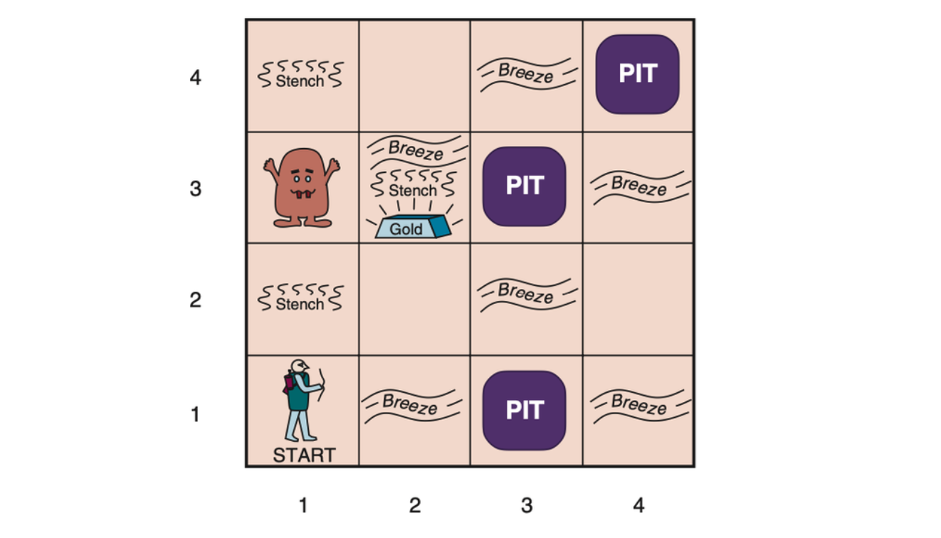
A typical wumpus world. The agent is in the bottom left corner, facing east (rightward).

Performance measure: +1000 for climbing out of the cave with the gold, –1000 for falling into a pit or being eaten by the wumpus, –1 for each action taken, and –10 for using up the arrow. The game ends either when the agent dies or when the agent climbs out of the cave.
Environment: A 4×4 grid of rooms, with walls surrounding the grid. The agent always starts in the square labeled [1,1], facing to the east. The locations of the gold and the wumpus are chosen randomly, with a uniform distribution, from the squares other than the start square. In addition, each square other than the start can be a pit, with probability 0.2.
Actuators: The agent can move Forward, TurnLeft by 90◦, or TurnRight by 90◦. The agent dies a miserable death if it enters a square containing a pit or a live wumpus. (It is safe, albeit smelly, to enter a square with a dead wumpus.) If an agent tries to move forward and bumps into a wall, then the agent does not move. The action Grab can be used to pick up the gold if it is in the same square as the agent. The action Shoot can be used to fire an arrow in a straight line in the direction the agent is facing. The arrow continues until it either hits (and hence kills) the wumpus or hits a wall. The agent has only one arrow, so only the first Shoot action has any effect. Finally, the action Climb can be used to climb out of the cave, but only from square [1,1].
Sensors: The agent has five sensors, each of which gives a single bit of information:
1. In the squares directly (not diagonally) adjacent to the wumpus, the agent will perceive a Stench.
2. In the squares directly adjacent to a pit, the agent will perceive a Breeze.
3. In the square where the gold is, the agent will perceive a Glitter.
4. When an agent walks into a wall, it will perceive a Bump.
5. When the wumpus is killed, it emits a woeful Scream that can be perceived anywhere in the cave.
The percepts will be given to the agent program in the form of a list of five symbols; for example, if there is a stench and a breeze, but no glitter, bump, or scream, the agent program will get [Stench, Breeze, None, None, None].

Two later stages in the progress of the agent. (a) After moving to [1,1] and then [1,2], and perceiving [Stench, None, None, None, None]. (b) After moving to [2,2] and then [2,3], and perceiving [Stench, Breeze, Glitter, None, None].

Logic

A logic must also define the semantics, or meaning, of sentences. The semantics defines the truth of each sentence with respect to each possible world. With more precision, the term model is used instead of “possible world”.

If a sentence \(\alpha\) is true in model \(m\), we say that \(m\) satisfies \(\alpha\) or sometimes \(m\) is a model of \(\alpha\). The notation \(M(\alpha)\) is used to mean the set of all models of \(\alpha\).

Logical entailment is defined as

\[ \alpha \models \beta \text{ if and only if } M(\alpha) \subseteq M(\beta) \]

which means \(\alpha \vDash \beta\) if and only if, in every model in which \(\alpha\) is true, \(\beta\) is also true. \(\alpha\) is a stronger assertion than \(\beta\).

If an inference algorithm \(i\) can derive \(\alpha\) from KB, we write

\[ KB \vdash_i \alpha \]

which is pronounced “\(\alpha\) is derived from KB by \(i\)” or “\(i\) derives \(\alpha\) from KB”.

An inference algorithm that derives only entailed sentences is call sound or truth preserving. An inference algorithm is complete if it can derive any sentence that is entailed.

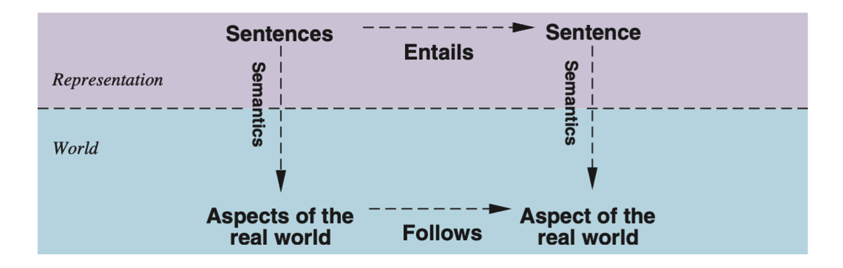
Sentences are physical configurations of the agent, and reasoning is a process of constructing new physical configurations from old ones. Logical reasoning should ensure that the new configurations represent aspects of the world that actually follow from the aspects that the old configurations represent.

The final issue to consider is grounding —— the connection between logical reasoning processes and the real environment in which the agent exists. In particular, how do we know that KB is true in the real world? A simple answer is that the agent’s sensors create the connection.

Propositional Logic: A Very Simple Logic

Syntax

The syntax of propositional logic defines the allowable sentences. The atomic sentences consist of a single proposition symbol. Each symbol stands for a proposition that can be true or false. There are two proposition symbols with fixed meanings: True is the always-true proposition and False is the always-false proposition.

Complex sentences are constructed from simpler sentences, using parentheses and operators called logical connectives.

\(\neg\) (not): A literal is either an atomic sentence (a positive literal) or a negated atomic sentence (a negative literal).
\(\land\) (and): A sentence whose main connective is \(\land\) is called a conjunction; its parts are the conjuncts.
\(\lor\) (or): A sentence whose main connective is \(\lor\) is a disjunction; its parts are disjuncts.
\(\implies\) (implies): Implications are also known as rules or if-then statements.
\(\iff\) (if and only if): The sentence \(A \iff B\) is biconditional.

Below gives the grammar of propositional logic.

A BNF (Backus–Naur Form) grammar of sentences in propositional logic, along with operator precedences, from highest to lowest.

\[ \begin{align*} \text{Sentence} &\to \text{AtomicSentence} | \text{ComplexSentence} \\ \text{AtomicSentence} &\to True | False | P | Q | R | \cdots \\ \text{ComplexSentence} &\to (\text{Sentence}) \\ &\ \ \ | \ \ \neg \text{Sentence} \\ &\ \ \ | \ \ \text{Sentence} \land \text{Sentence} \\ &\ \ \ | \ \ \text{Sentence} \lor \text{Sentence} \\ &\ \ \ | \ \ \text{Sentence} \implies \text{Sentence} \\ &\ \ \ | \ \ \text{Sentence} \iff \text{Sentence} \\ \text{Operator Precedence} &\ \ : \ \ \neg, \land, \lor, \implies, \iff \end{align*} \]

Semantics

In propositional logic, a model simply set the truth value —— true or false —— for every proposition symbol. The semantics for propositional logic must specify how to compute the truth value of any sentence, given a model.

Rules for evaluating atomic sentences.

True is true in every model and False is false in every model.
The truth value of every other proposition symbol must be specified directly in the model.

For complex sentences, the following rules hold for subsentences \(P\) and \(Q\) in any model \(m\).

\(\neg P\) is true iff \(P\) is false in \(m\).
\(P \land Q\) is true iff both \(P\) and \(Q\) are true in \(m\).
\(P \lor Q\) is true iff either \(P\) or \(Q\) are true in \(m\).
\(P \implies Q\) is true unless \(P\) is true and \(Q\) is false in \(m\).
\(P \iff Q\) is true iff \(P\) and \(Q\) are both true or both false in \(m\).

\(P\)	\(Q\)	\(\neg P\)	\(P \land Q\)	\(P \lor Q\)	\(P \implies Q\)	\(P \iff Q\)
false	false	true	false	false	true	true
false	true	true	false	true	true	false
true	false	false	false	true	false	false
true	true	false	true	true	true	true

Truth tables for the five logical connectives. To use the table to compute, forexample, the value of P ∨ Q when P is true and Q is false, first look on the left for the row where P is true and Q is false (the third row). Then look in that row under the P ∨ Q column to see the result: true.

A Simple Knowledge Base

For the wumpus world, define the following symbols for each \([x, y]\) location:

\(P_{x, y}\) is true if there is a pit in \([x, y]\).
\(W_{x, y}\) is true if there is a wumpus in \([x, y]\), dead or alive.
\(B_{x, y}\) is true if there is a breeze in \([x, y]\).
\(S_{x, y}\) is true if there is a stench in \([x, y]\).
\(L_{x, y}\) is true if the agent is in location \([x, y]\).

Sentences in the knowledge base of the wumpus world are something like

There is no pit in \([1, 1]\):

\[ R_1: \neg P_{1, 1} \]
A square is breezy if and only if there is a pit in a neighboring square.

\[ \begin{align*} R_2 &: B_{1, 1} \iff (P_{1, 2} \lor P_{2, 1}) \\ R_3 &: B_{2, 1} \iff (P_{1, 1} \lor P_{2, 2} \lor P_{3, 1}) \\ \end{align*} \]
The breeze percepts for the first two squares visisted in the specific world the agent is in, leading up to the situation in the above figure (b).

\[ \begin{align*} R_4 &: \neg B_{1, 1} \\ R_5 &: B_{2, 1} \end{align*} \]

A Simple Inference Procedure

The goal now is to decide whether \(KB \models \alpha\) for some sentence \(\alpha\). A basic algorithm for inference is a model-checking approach that is a direct implementation of the definition of entailment: enumerate the models, and check that \(\alpha\) is true in every model in which \(KB\) is true. Models are assignments of true or false to every proposition symbol.

\(B_{1, 1}\)	\(B_{2, 1}\)	\(P_{1, 1}\)	\(P_{1, 2}\)	\(P_{2, 1}\)	\(P_{2, 2}\)	\(P_{3, 1}\)	\(R_1\)	\(R_2\)	\(R_3\)	\(R_4\)	\(R_5\)	KB
false	false	false	false	false	false	false	true	true	true	true	false	false
false	false	false	false	false	false	true	true	true	false	true	false	false
\(\vdots\)	\(\vdots\)	\(\vdots\)	\(\vdots\)	\(\vdots\)	\(\vdots\)	\(\vdots\)	\(\vdots\)	\(\vdots\)	\(\vdots\)	\(\vdots\)	\(\vdots\)	\(\vdots\)
false	true	false	false	false	false	true	true	true	false	true	true	false
false	true	false	false	false	false	true	true	true	true	true	true	true
false	true	false	false	false	true	false	true	true	true	true	true	true
false	true	false	false	false	true	true	true	true	true	true	true	true
false	true	false	false	true	false	false	true	false	false	true	true	false
\(\vdots\)	\(\vdots\)	\(\vdots\)	\(\vdots\)	\(\vdots\)	\(\vdots\)	\(\vdots\)	\(\vdots\)	\(\vdots\)	\(\vdots\)	\(\vdots\)	\(\vdots\)	\(\vdots\)
true	true	true	true	true	true	true	false	true	true	false	true	false

A truth table constructed for the knowledge base given in the text. KB is true if R1 through R5 are true, which occurs in just 3 of the 128 rows (the ones underlined in the right-hand column). In all 3 rows, P1,2 is false, so there is no pit in [1,2]. On the other hand, there might (or might not) be a pit in [2,2].

function TT_Entails(
    // knowledge base, a sentence in propositional logic
    KB: KnowledgeBase,
    // the query, a sentence in propositional logic
    a: Query
): boolean {
    const symbols = [
        ...KB.propositionSymbols(),
        ...a.propositionalSymbols()
    ]
    return TT_CheckAll(KB, a, symbols, new Set())
}

function TT_CheckAll(KB: KnowledgeBase, a: Query, symbols, model): boolean {
    if (symbols.length === 0) {
        if (PL_True(KB, model)) return PL_True(a, model)
        return true // when KB is false, always return true
    } else {
        const [P, ...rest] = symbols
        return TT_CheckAll(KB, a, rest, AND(model, True(P)))
            && TT_CheckAll(KB, a, rest, AND(model, False(P)))
    }
}

A truth-table enumeration algorithm for deciding propositional entailment. (TT stands for truth table.) PL-TRUE? returns true if a sentence holds within a model. The variable model represents a partial model —— an assignment to some of the symbols. The keyword and here is an infix function symbol in the pseudocode programming language, not an operator in propositional logic; it takes two arguments and returns true or false.

Propositional Theorem Proving

Entailment can be done by theorem proving —— applying rules of inference directly to the sentences in our knowledge base to construct a proof of the desired sentence without consulting models. If the number of models is large but the length of the proof is short, then theorem proving can be more efficient than model checking.

Two sentences \(\alpha\) and \(\beta\) are logically equivalent if they are true in the same set of models. We write this as \(\alpha \equiv \beta\). Any two sentences \(\alpha\) and \(\beta\) are equivalent if and only if each of them entails the other:

\[ \alpha \equiv \beta \text{ if and only if } \alpha \models \beta \text{ and } \beta \models \alpha \]

A sentence is valid if it is true in all models. For example, the sentence \(P \lor \neg P\) is valid. Valid sentences are also known as tautologies —— they are necessarily true.

Deduction theorem:

\[ \forall \alpha, \forall \beta, \alpha \models \beta \text{ if and only if the sentence } (\alpha \implies \beta) \text{ is valid.} \]

Hence, we can decide if \(\alpha \models \beta\) by checking that \((\alpha \implies \beta)\) is true in every model.

A sentence is satisfiable if it is true in, or satisfied by, some model. Satisfiability can be checked by enumerating the possible models until one is found that satisfies the sentence. The problem of determining the satisfiability of sentences in propositional logic —— the SAT problem —— was the first problem proved to be NP-complete.

Validity and satisfiability are connected: \(\alpha\) is valid iff \(\neg \alpha\) is unsatisfiable. A useful result is given below:

\[ \alpha \models \beta \text{ if and only if the sentence} (\alpha \land \neg \beta) \text{ is unsatisfiable.} \]

Proving \(\beta\) from \(\alpha\) by checking the unsatisfiability of \((\alpha \land \neg \beta)\) corresponds exactly to the standard mathematical proof technique of refutation or proof by contradiction.

Inference and Proofs

Inference rules can be applied to derive a proof —— a chain of conclusions that leads to the desired goal. The best-known rule is called Modus Ponens and is written

\[ \frac{\alpha \implies \beta, \alpha}{\beta} \]

which means that, whenever any sentences of the form \(\alpha \implies \beta\) and \(\alpha\) is given, then the sentence \(\beta\) can be inferred.

Another useful inference rule is And-Elimination, which says that, from a conjunction, any of the conjuncts can be inferred.

\[ \frac{\alpha \land \beta}{\alpha} \]

Standard logical equivalences are shown as below

\[ \begin{align*} (\alpha \land \beta) &\equiv (\beta \land \alpha) &\text{ community of } \land \\ (\alpha \lor \beta) &\equiv (\beta \lor \alpha) &\text{ community of } \lor \\ ((\alpha \land \beta) \land \gamma) &\equiv (\alpha \land (\beta \land \gamma)) &\text{ associativity of } \land \\ ((\alpha \lor \beta) \lor \gamma) &\equiv (\alpha \lor (\beta \lor \gamma)) &\text{ associativity of } \lor \\ \neg(\neg \alpha) &\equiv \alpha &\text{ double-negation elimination} \\ (\alpha \implies \beta) &\equiv (\neg \beta \implies \neg \alpha) &\text{ contraposition} \\ (\alpha \implies \beta) &\equiv (\neg \alpha \lor \beta) &\text{ implication elimination} \\ (\alpha \iff \beta) &\equiv ((\alpha \implies \beta) \land (\beta \implies \alpha)) &\text{ biconditional elimination} \\ \neg (\alpha \land \beta) &\equiv (\neg \alpha \lor \neg \beta) &\text{De Morgan} \\ \neg (\alpha \lor \beta) &\equiv (\neg \alpha \land \neg \beta) &\text{De Morgan} \\ (\alpha \land (\beta \lor \gamma)) &\equiv ((\alpha \land \beta) \lor (\beta \land \gamma)) &\text{distributivity of } \land \text{ over } \lor \\ (\alpha \lor (\beta \land \gamma)) &\equiv ((\alpha \lor \beta) \land (\beta \lor \gamma)) &\text{distributivity of } \lor \text{ over } \land \end{align*} \]

The symbols \(\alpha\), \(\beta\) and \(\gamma\) stand for arbitrary sentences of propositional logic. All the logical equivalences can be used as inference rules.

Any of the search algorithms can be used to find a sequence of steps that constitutes the proof. The proof problem can be defined as:

Initial State: the initial knowledge base.
Actions: the set of actions consists of all the inference rules applied to all the sentences that match the top half of the inference rule.
Result: the result of an action is to add the sentence in the bottom half of the inference rule.
Goal: the goal is a state that contains the sentence we are trying to prove.

One final property of logical systems is monotonicity, which says that the set of entailed sentences can only increase as information is added to the knowledge base. For any sentences \(\alpha\) and \(\beta\),

\[ \text{ if } KB \models \alpha \text{ then } KB \land \beta \models \alpha \]

Monotonicity means that inference rules can be applied whenever suitable premises are found in the knowledge base —— the conclusion of the rule must folow regardless of what else is in the knowledge base.

Proof by Resolution

A inference rule, resolution, that can yield a complete inference algorithm when coupled with any complete search algorithm.

The unit resolution inference rule is defined as below:

\[ \frac{l_1 \lor \cdots \lor l_k, \ m}{l_1 \lor \cdots \lor l_{i - 1} \lor l_{i + 1} \lor \cdots \lor l_k} \]

where each \(l\) is a literal and \(l_i\) and \(m\) are complementary literals (one is the negation of the other). The unit resolution rule can be generalized to the full resolution rule.

\[ \frac{l_1 \lor \cdots \lor l_k, \ m_1 \lor \cdots m_n}{l_1 \lor \cdots \lor l_{i - 1} \lor l_{i + 1} \lor \cdots \lor l_k \lor m_1 \lor \cdots \lor m_{j - 1} \lor m_{j + 1} \lor \cdots \lor m_n} \]

where \(l_i\) and \(m_j\) are complementary literals. The resulting clause should contain only one copy of each literal. The removal of multiple copies of literals is called factoring. For example, if we resolve \((A \lor B)\) with \((A \lor \neg B)\), we obtain \((A \lor A )\), which is reduced to just \(A\) by factoring.

Conjunctive Normal Form

Every sentence of propositional logic (that is, disjunctions of literals) is logically equivalent to a conjunction of clauses. A sentence expressed as a conjunction of clauses is said to be in conjunctive normal form or CNF.

\[ \begin{align*} \text{CNFSentence} &\to \text{Clause}_1 \land \cdots \land \text{Clause}_n \\ \text{Clause} &\to \text{Literal}_1 \lor \cdots \lor \text{Literal}_m \\ \text{Fact} &\to \text{Symbol} \\ \text{Literal} &\to \text{Symbol} \ | \ \neg \text{Symbol} \\ \text{Symbol} &\to P \ |\ Q \ |\ R \\ \text{HornClauseForm} &\to \text{DefiniteClauseForm} \ | \ \text{GoalClauseForm} \\ \text{DefiniteClauseForm} &\to \text{Fact} \ | \ (\text{Symbol}_1 \land \cdots \land \text{Symbol}_l) \implies \text{Symbol} \\ \text{GoalClauseForm} &\to (\text{Symbol}_1 \land \cdots \land \text{Symbol}_l) \implies \text{False} \\ \end{align*} \]

A grammar for conjunctive normal form, Horn clauses, and definite clauses. A CNF clause such as \(\neg A \lor \neg B \lor C\) can be written in definite clause form as \(A \land B \implies C\).

Example: converting the sentence \(B_{1, 1} \iff (P_{1, 2} \lor P_{2, 1})\) into CNF.

Eliminate \(\iff\), replacing \(\alpha \iff \beta\) with \((\alpha \implies \beta) \land (\beta \implies \alpha)\):

\((B_{1, 1} \implies (P_{1, 2} \lor P_{2, 1})) \land ((P_{1, 2} \lor P_{2, 1}) \implies B_{1, 1})\)
Eliminate \(\implies\), replacing \(\alpha \implies \beta\) with \(\neg \alpha \lor \beta\):

\((\neg B_{1, 1} \lor P_{1, 2} \lor P_{2, 1}) \land (\neg(P_{1, 2} \lor P_{2, 1}) \lor B_{1, 1})\)
CNF requires \(\neg\) to appear only in literals, so repeatedly using double-negation elimination and De Morgan to move \(\neg\) inwards.

\((\neg B_{1, 1} \lor P_{1, 2} \lor P_{2, 1}) \land ((\neg P_{1, 2} \land \neg P_{2, 1}) \lor B_{1, 1})\)
Then apply the distributivity law to further reduce nested \(\lor\) and \(\land\).

\((\neg B_{1, 1} \lor P_{1, 2} \lor P_{2, 1}) \land (\neg P_{1, 2} \lor B_{1, 1}) \land (\neg P_{2, 1} \lor B_{1, 1})\) >

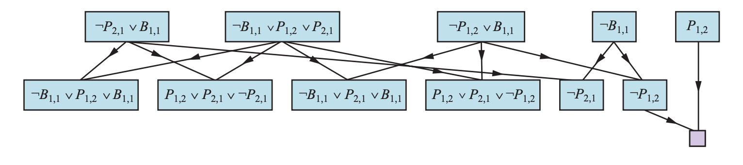
A Resolution Algorithm

Inference procedures based on resolution work by using the principle of proof by contradiction. That is, to show that \(KB \models \alpha\), we show that \((KB \land \neg \alpha)\) is unsatisfiable.

First, \((KB \land \neg \alpha)\) is converted to CNF. Then, the resolution rule is applied to the resulting clauses. Each pair that contains complementary literals is resolved to produce a new clause, which is added to the set if it is not already present. The process continues until one of the two things happens:

there are no new clauses that can be added, in which case \(KB\) does not entail \(\alpha\).
two clauses resolve to yield the empty clause, in which case \(KB\) entails \(\alpha\).

function PL_Resolution(KB: KnowledgeBase, a: Query): boolean {
    // the set of clauses in the CNF representation of KB ∧ ¬α
    let clauses = new CNF(AND(KB, NOT(a))).clauses()
    let sentences = new Set()

    while (true) {
        clauses.forEach((Ci, Cj) => {
            const resolvents = PL_Resolve(Ci, Cj)
            if (Resolvents.includes(EmptyClause)) return true
            sentences = Union(sentences, resolvents)
        })

        if (clauses.contains(sentences)) return false
        clauses = Union(clauses, sentences)
    }
}

PL-RESOLVE returns the set of all possible clauses obtained by resolving its two inputs.

Partial application of PL-RESOLUTION to a simple inference in the wumpus world to prove the query ¬P1,2. Each of the leftmost four clauses in the top row is paired with each of the other three, and the resolution rule is applied to yield the clauses on the bottom row. We see that the third and fourth clauses on the top row combine to yield the clause ¬P1,2, which is then resolved with P1,2 to yield the empty clause, meaning that the query is proven.

Completeness of Resolution

The algorithm PL-RESOLUTION is complete. Define resolution closure \(RC(S)\) of a set of clauses \(S\), which is the set of all clauses derivable by repeated application of the resolution rule to clauses in \(S\) or their derivatives. The resolution closure is what PL-RESOLUTION computes as the final value of the variable clauses. Thanks to the factoring step, there are only finitely many distinct clauses that can be constructed out of the symbols \(P_1, \dots, P_k\) that appear in \(S\). Hance, PL-RESOLUTION always terminates.

The completeness theorem for resolution in propositional logic is called the ground resolution theorem:

\[ \text{ If a set of clauses is unsatisfiable, then the} \\ \text{ resolution closure of those clauses contains the empty clause} \]

Horn Clauses and Definite Clauses

Definite clause is a disjunction of literals of which exactly one is positive. Slightly more general is the Horn clause, which is a disjunction of literals of which at most one is positive. So all definite clauses are Horn clauses. Goal clauses are those with no positive literals. \(k\)-CNF sentence is a CNF sentence where each clause has at most \(k\) literals.

Knowledge bases containing only definite clauses are interesting for three reasons:

Every definite clause can be written as an implication whose premise is a conjunction of positive literals and whose conclusion is a single positive literal. For example, the definite clause \((\neg L_{1, 1} \lor \neg Breeze \lor B_{1, 1})\) can be written as the implication \((L_{1, 1} \land Breeze) \implies B_{1, 1}\). In Horn form, the premise is called the body and the conclusion is called the head. A sentence consisting of a single positive literal is called a fact.
Inference with Horn clauses can be done throught the forward-chaining and backward-chaining.
Deciding entailment with Horn clauses can be done in time that is linear in the size of the knowledge base.

Forward and Backward Chaining

The forward-chaining algorithm PL-FC-ENTAILS?(KB, q) determines if a single proposition symbol \(q\) —— the query —— is entail by a knowledge base of definite clauses.

// Forward-chaining Algorithm
function PL_FC_Entails(KB: KnowledgeBase, q: Query): boolean {
    // a table, where count[c] is initially the number of
    // symbols in clause c’s premise
    const count = {}
    // a table, where inferred[s] is initially false for all symbols
    const inferred = {}
    // a queue of symbols, initially symbols known to be true in KB 
    const queue = KB.trueSymbols()

    while (queue.length > 0) {
        const p = queue.pop()
        if (p === q) return true
        if (!inferred[p]) {
            inferred[p] = true
            KB.clauses.forEach(clause => {
                if (clause.premise.includes(p)) {
                    count[clause] -= 1
                    if (count[clause] === 0) {
                        queue.push(c.conclusion)
                    }
                }
            })
        }
    }

    return false
}

The forward-chaining algorithm for propositional logic. The queue keeps track of symbols known to be true but not yet “processed.” The count table keeps track of how many premises of each implication are not yet proven. Whenever a new symbol p from the agenda is processed, the count is reduced by one for each implication in whose premise p appears (easily identified in constant time with appropriate indexing.) If a count reaches zero, all the premises of the implication are known, so its conclusion can be added to the agenda. Finally, we need to keep track of which symbols have been processed; a symbol that is already in the set of inferred symbols need not be added to the agenda again. This avoids redundant work and prevents loops caused by implications such as \(p \implies Q\) and \(Q \implies P\).

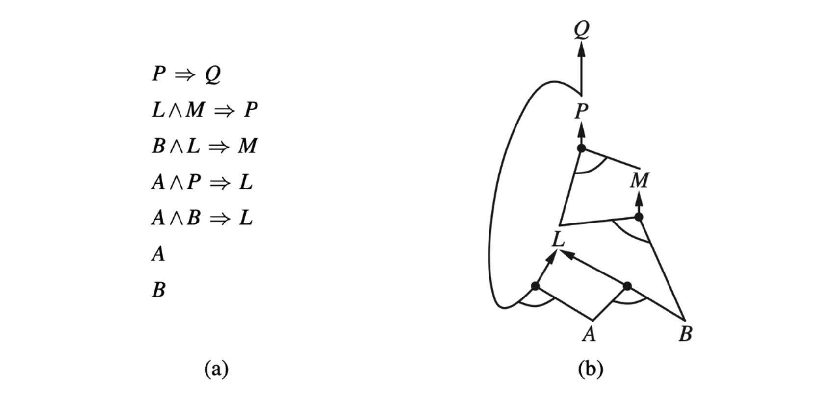
(a) A set of Horn clauses. (b) The corresponding AND–OR graph.

A set of Horn clauses. (b) The corresponding AND–OR graph.

Forward chaining is an example of the general concept of data-driven reasoning —— that is, reasoning in which the focus of attention starts with the known data. It can be used within an agent to derive conclusions from incoming percepts, often without a specific query in mind.

Effective Propositional Model Checking

A Complete Backtracking Algorithm

DPLL takes an input a sentence in conjunctive normal form —— a set of clauses. It embodies three improvements over the simple scheme of TT-ENTAILS?.

Early termination: The algorithm detects whether the sentence must be true or false, even with a partially completed model.
Pure symbol heuristic: A pure symbol is a symbol that always appears with the same “sign” in all clauses.
Unit clause heuristic: A unit clause was defined earlier as a clause with just one literal. In the context of DPLL, it also means clauses in which all literals but one are already assigned false by the model.

// Forward-chaining Algorithm
function DPLL_Statisfiable(s: Sentence): boolean {
    const clauses = new CNF(s).clauses()
    const symbols = s.propositionSymbols()
    return DPLL(clauses, symbols, new Set())
}

function DPLL(clauses, symbols, model): boolean {
    const allTrue = _.every(clauses, clause => model.check(clause))
    if (allTrue) return true
    const someFalse = _.some(clauses, clause => !model.check(clause))
    if (someFalse) return false

    let [P, value] = FindPureSymbol(symbols, clauses, model)
    if (P) return DPLL(clauses, _.omit(symbols, P), Union(model, Value(P)))

    let [P, value] = FindUnitClause(clauses, model)
    if (P) return DPLL(clauses, _.omit(symbols, P), Union(model, Value(P)))

    let [P, ...rest] = symbols
    return DPLL(clauses, rest, Union(model, True(P)))
        || DPLL(clauses, rest, Union(model, False(P)))
}

Agents based on Propositional Logic

The Current State of the World

The knowledge base is composed of axioms —— general knowledge about how the world works —— and percept sentences obtained from the agent’s experience in a particular world.

For each square, it knows that the square is breezy if and only if a neighboring square has a pit; and a square is smelly if and only if a neighboring square has a wumpus. In such a way, a large collection of axioms can be included.

\[ \begin{align*} B_{1, 1} &\iff (P_{1, 2} \lor P_{2, 1}) \\ S_{1, 1} &\iff (W_{1, 2} \lor W_{2, 1}) \\ &\ \ \ \ \ \vdots \end{align*} \]

The agent also knows that there is exactly one wumpus. First, we have to say that there is at least one wumpus.

\[ W_{1, 1} \lor W_{1, 2} \lor \cdots \lor W_{4, 3} \lor W_{4, 4} \]

Then we have to say that there is at most one wumpus.

\[ \begin{align*} \neg W_{1, 1} &\lor \neg W_{1, 2} \\ \neg W_{1, 1} &\lor \neg W_{1, 3} \\ &\ \vdots \\ \neg W_{4, 3} &\lor \neg W_{4, 4} \\ \end{align*} \]

The idea of associating propositions with time steps extends to any aspect of the world that changes over time. For example, the initial knowledge base includes \(L^0_{1, 1}\) —— the agent is in square \([1, 1]\) at time 0 —— as well as \(FacingEast^0\), \(HaveArrow^0\), and \(WumpusAlive^0\). We use the noun fluent to refer to an aspect of the world that changes. “Fluent” is a synonym for “state variable”.

We can connect stench and breeze percepts directly to the properties of the squares where they are experienced as follows. For any time step \(t\) and any square \([x, y]\), we assert

\[ L^t_{x, y} \implies (Breeze^t \iff B_{x, y}) \\ L^t_{x, y} \implies (Stench^t \iff S_{x, y}) \]

Then we need axioms that allow the agent to keep track of fluents such as \(L^t_{x, y}\). These fluents change as the result of actions taken by the agent. To describe how the world changes, we can try writing effect axioms that specify the outcome of an action at the next time step. For example, if the agent is at location \([1, 1]\) facing east at time 0 and goes \(Forward\), the result is that the agent is in square \([2, 1]\):

\[ L^0_{1, 1} \land FacingEast^0 \land Forward^0 \implies (L^1_{2, 1} \land \neg L^1_{1, 1}) \]

We would need one such sentence for each possible time step, for each of the 16 squares, and each of the four orientations. We would also need similar sentences for the other actions: \(Grab\), \(Shoot\), \(Climb\), \(TurnLeft\), \(TurnRight\).

There is some information that remains unchanged as the result of an action. The need to do this gives rise to the frame problem. One possible solution to the frame problem would be to add frame axioms explicitly asserting all propositions that remain the same. For example, for each time \(t\) we have

\[ \begin{align*} Forward^t &\implies (HaveArrow^t \iff HaveArrow^{t + 1}) \\ Forward^t &\implies (WumpusAlive^t \iff WumpusAlive^{t + 1}) \\ &\ \ \ \ \ \vdots \end{align*} \]

In a world with \(m\) different actions and \(n\) fluents, the set of frame axioms will be of size \(O(mn)\). The solution to the problem involves changing one’s focus from writing axioms about actions to writing axioms about fluents.

For each fluent \(F\), we will have an axiom that defines the truth value of \(F^{t + 1}\) in terms of fluents at time \(t\) and the actions that may have occurred as time \(t\). The following is a successor-state axiom:

\[ F^{t + 1} \iff ActionCausesF^t \lor (F^t \land \neg ActionCausesNotF^t) \]

The successor-state axiom for \(HaveArrow\) is as follows.

\[ HaveArrow^{t + 1} \iff (HaveArrow^t \land \neg Shoot^t) \]

For the agent’s location, the successor-state axioms are more elaborate.

\[ \begin{align*} L^{t+1}_{1, 1} &\iff (L^t_{1, 1} \land (\neg Forward^t \lor Bump^{t + 1})) \\ &\lor (L^t_{1, 2} \land (FacingSouth^t \land Forward^t)) \\ &\lor (L^t_{2, 1} \land (FacingWest^t \land Forward^t)) \\ \end{align*} \]

The most important question for the agent is whether a square is OK to move into —— that is, whether the square is free of a pit or live wumpus. It’s coinvenient to add axioms for this

\[ OK^t_{x, y} \iff \neg P_{x, y} \land \neg(W_{x, y} \land WumpusAlive^t) \]

So finally, the agent can move into any square where \(\text{ASK}(KB, OK^t_{x, y}) = true\).

A hybrid agent

The agent program maintains and updates a knowledge base as well as a current plan. The initial knowledge base contains atemporal axioms —— those that don’t depend on \(t\), such as the successor-state axioms. At each time step, the new percept sentence is added along with all the axioms that depend on \(t\), such as the successor-state axioms.

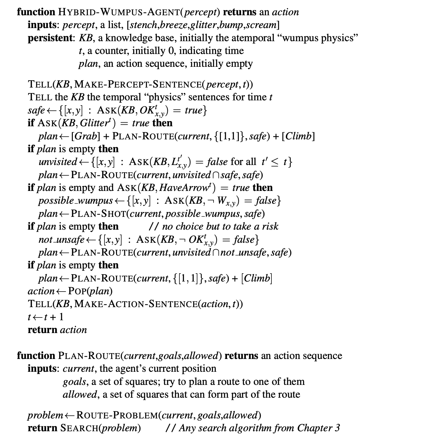
The main body of the agent program constructs a plan based on a decreasing priority of goals. First, if there is a glitter, the program constructs a plan to grab the gold, follow a route back to the initial location, and climb out of the cave. Otherwise, if there is no current plan, the program plans a route to the closest safe square that it has not visited yet, making sure the route goes through only safe squares.