Search in Complex Environments

发表于 2023-03-25 分类于 Reading Disqus：本文字数： 3k 阅读时长 ≈ 11 分钟

Local Search and Optimization Problems

Local search algorithms operate by searching from a start state to neighboring states, without keeping track of the paths, nor the set of states that have been reached. They have two key advantages:

They use very little memory.
They can often find reasonable solutions in large or infinite state spaces for which systematic algorithms are unsuitable.

Local search algorithms can also solve optimization problems, in which the aim is to find the best state according to an objective function.

Consider the state of a problem laid out in a state-space landscape.

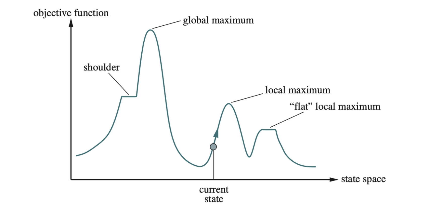
A one-dimensional state-space landscape in which elevation corresponds to the objective function. The aim is to find the global maximum.

then the aim is to find the highest peak—a global maximum—and we call the process hill climbing. If elevation corresponds to cost, then the aim is to find the lowest valley—a global minimum—and we call it gradient descent.

Hill-Climbing Search

The hill-climbing search algorithm keeps track of one current state and on each iteration moves to the neighboring state with highest value —— that is, it heads in the direction that provides the steepest ascent.

// Hill-Climbing Search Algorithm
function HillClimbing(problem: Problem): State {
    let current = problem.initial
    while (true) {
        const neighbor = HighestValuedSuccessorState(current)
        if (Value(neighbor) <= Value(current)) return current
        current = neighbor
    }
}

Hill climbing is sometimes called greedy local search. It can get stuck for any of the following reasons:

Local maxima: A local maximum is a peak that is higher than each of its neighboring states but lower than the global maximum. Hill-climbing algorithms that reach the vincity of a local maximum will be drawn upward toward the peak but will then be stuck with nowhere else to go.
Ridges: Ridges result in a sequence of local maxima that is very difficult for greedy algorithms to navigate.
Plateaus: A plateau is a flat area of the state-space landscape. It can be a flat local maximum, from which no uphill exit exists, or a shoulder, from which progress is possible. A hill-climbing search can get lost wandering on the plateau.

Illustration of why ridges cause difficulties for hill climbing. The grid of states (dark circles) is superimposed on a ridge rising from left to right, creating a sequence of local maxima that are not directly connected to each other. From each local maximum, all the available actions point downhill. Topologies like this are common in low-dimensional state spaces, such as points in a two-dimensional plane. But in state spaces with hundreds or thousands of dimensions, this intuitive picture does not hold, and there are usually at least a few dimensions that make it possible to escape from ridges and plateaus.

Many variants of hill climbing have been invented.

Stochastic hill climbing: chooses at random from among the uphill moves; the probability of selection can vary with the steepness of the uphill move.
First-choice hill climbing: implements stochastic hill climbing by generating successors randomly until one is generated that is better than the current state.
Random-restart hill climbing: which conducts a series of hill-climbing searches from randomly generated initial states, until a goal is found.

Simulated Annealing

It seems reasonable to try to combine hill climbing with a random walk in a way that yields both efficiency and completeness. The overall structure of the simulated-annealing algorithm is similar to hill climbing. Instead of picking the best move, however, it picks a random move. If the move improves the situation, it is always accepted. Otherwise, the algorithm accepts the move with some probability less than 1. The probability decreases exponentially with the “badness” of the move —— the amount \(\Delta E\) by which the evaluation is worsened. The probability also decreases as the “temperature” \(T\) goes down: “bad” moves are more likely to be allowed at the start when \(T\) is high, and they become more unlikely as \(T\) decreases. If the schedule lowers \(T\) to \(0\) slowly enough, then a property of the Boltzmann distribution, \(e^{\Delta E / T}\), is that all the probability is concentrated on the global maxima, which the algorithm will find with probability approaching 1.

// Simulated-Annealing Algorithm
function SimulatedAnnealing(problem: Problem, schedule): State {
    let current = problem.initial
    let t = 0
    while (true) {
        t += 1
        const T = schedule(t)
        if (T === 0) return current
        const next = RandomlySelectedSuccessor(current)
        const deltaE = Value(current) - Value(next)
        if (deltaE > 0) {
            current = next
        } else if (Math.random() < Math.pow(Math.E, deltaE / T)) {
            current = next
        }
    }
}

The schedule input determines the value of the “temperature” \(T\) as a function of time.

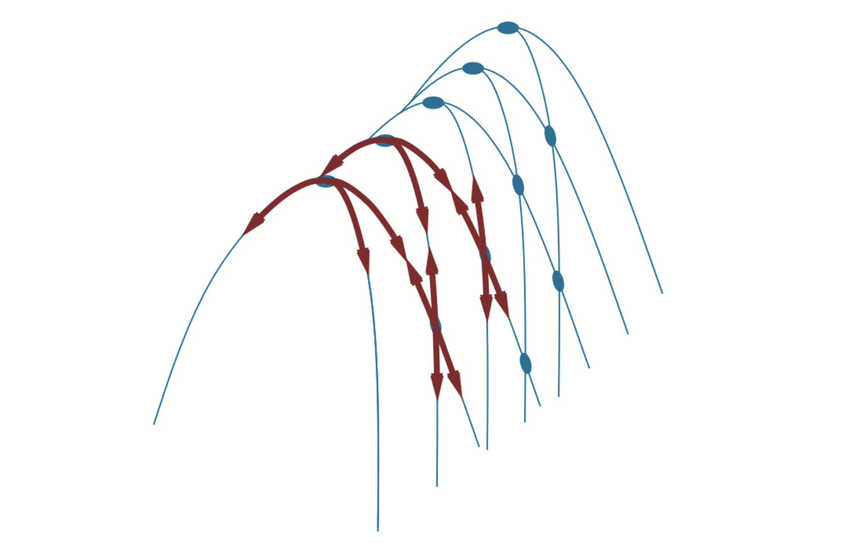
Local Beam Search

The local beam search algorithm keeps track of \(k\) states rather than just one. It begins with \(k\) randomly generated states. At each step, all the successors of all \(k\) states are generated. If any one is a goal, the algorithm halts. Otherwise, it selects the \(k\) best successors from the complete list and repeats.

Evolutionary Algorithms

Evolutionary algorithms can be seen as variants of stochastic beam search that are explicitly motivated by the metaphor of natural selection in biology: there is a population of individuals (states), in which the fittest (highest value) individuals produce offspring (successor states) that populate the next generation, a process called recombination.

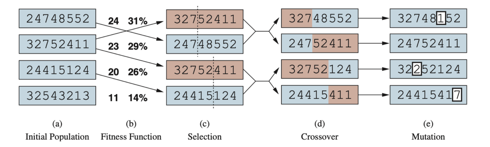
A genetic algorithm, illustrated for digit strings representing 8-queens states. The initial population in (a) is ranked by a fitness function in (b) resulting in pairs for mating in (c). They produce offspring in (d), which are subject to mutation in (e).

There are endless forms of evolutionary algorithms, varying in the following ways:

The size of population.
The representation of each individual. In genetic algorithms, each individual is a string over a finite alphabet (often a Boolean string). In genetic programming an individual is a computer program.
The mixing number, \(\rho\), which is the number of parents that come together to form offspring. The most common case is \(\rho = 2\): two parents combine their “genes” to form offspring.
The selection process for selecting the individuals who will become the parents of the next generation.
The recombination procedure. One common approach is to randomly select a crossover point to split each of the parent strings, and recombine the parts to form two children.
The mutation rate, which determines how often offspring have random mutations to their representation.
The makeup of the next generation. It can include a few top-scoring parents from the previous generation (elitism). The practice of culling, in which all individuals below a given threshold are discarded, can lead to a speedup.

// Genetic Algorithm
function GeneticAlgorithm(population, fitness): Individual {
    do {
        const weights = WeightedBy(population, fitness)
        const population2 = []
        for (let i = 0; i < population.size(); ++i) {
            const [parent1, parent2] = RandomChoices(population, weights, 2)
            let child = Reproduce(parent1, parent2)
            if (SmallRandomProbability) {
                child = Mutate(child)
            }
            population2.push(child)
        }
        population = population2
    } while (SomeIndividualIsFitEnough || EnoughTimeHasElapsed)

    return population.best({ orderBy: fitness })
}

function Reproduce(parent1, parent2): Individual {
    const n = parent1.length
    const c = Random(1, n)
    return [
        parent1.substring(1, c),
        parent2.substring(c + 1, n)
    ].join('')
}

Genetic algorithms work best when schemas correspond to meaningful components of a solution.

Local Search in Continuous Spaces

A continuous action space has an infinite branching factor. In general, states are defined by an \(n\)-dimensional vector of variables, \(\textbf{x}\). One way to deal with a continuous state space is to discretize it.

Methods that measure progress by the change in the value of the objective function between two nearby points are called empirical gradient methods. Empirical gradient search is the same as steepest-ascent hill climbing in a discretized version of the state space.

Often we have an objective function expressed in a mathematical form such that we can use calculus to solve the problem by analytically rather than empirically. Many methods attempt to use the gradient of the landscape to find a maximum. The gradient of the objective function is a vector \(\nabla f\) that gives the magnitude and direction of the steepest slope.

In some cases, we can find a maximum by solving the equation \(\nabla f = 0\).

For many problems, the most effective algorithm is the Newton-Raphson method. This is a general technique for finding roots of functions —— that is, solving equations of the form \(g(x) = 0\). It works by computing a new estimate for the root \(x\) according to Newton’s formula

\[ x \gets x - g(x)/g'(x) \]

To find a maximum or minimum of \(f\), we need to find \(\textbf{x}\) such that the gradient is a zero vector. Thus the update equation becomes

\[ \textbf{x} \gets \textbf{x} - \textbf{H}_f^{-1}(\textbf{x})\nabla f(\textbf{x}) \]

where \(\textbf{H}_f(\textbf{x})\) is the Hessian matrix of second derivatives, whose elements \(H_{ij}\) are given by \(\partial^2 f / \partial x_i \partial x_j\).

An optimization problem is constrained if solutions must satisfy some hard constraints on the values of the variables. The best-known category is that of linear programming problems, in which constriants must be linear inequalities forming a convex set and the objective function is also linear.

Search with Nondeterministic Actions

When the environment is nondeterministic, the agent doesn’t know what state it transitions to after taking an action. That means that rather then thinking “I’m in state \(s_1\) and if I do action \(a\) I’ll end up in state \(s_2\)” an agent will now be thinking “I’m either in state \(s_1\) or \(s_3\), and if I do action \(a\) I’ll end up in state \(s_2, s_4\) or \(s_5\)”.

A set of physical states that the agent believes are possible a belief state. In partially observable and nondeterministic environments, the solution to a problem is no longer a sequence, but rather a conditional plan that specifies what to do depending on what percepts agent receives while executing the plan.

A conditional plan can contain if-then-else steps; this means that solutions are trees rather than sequences.

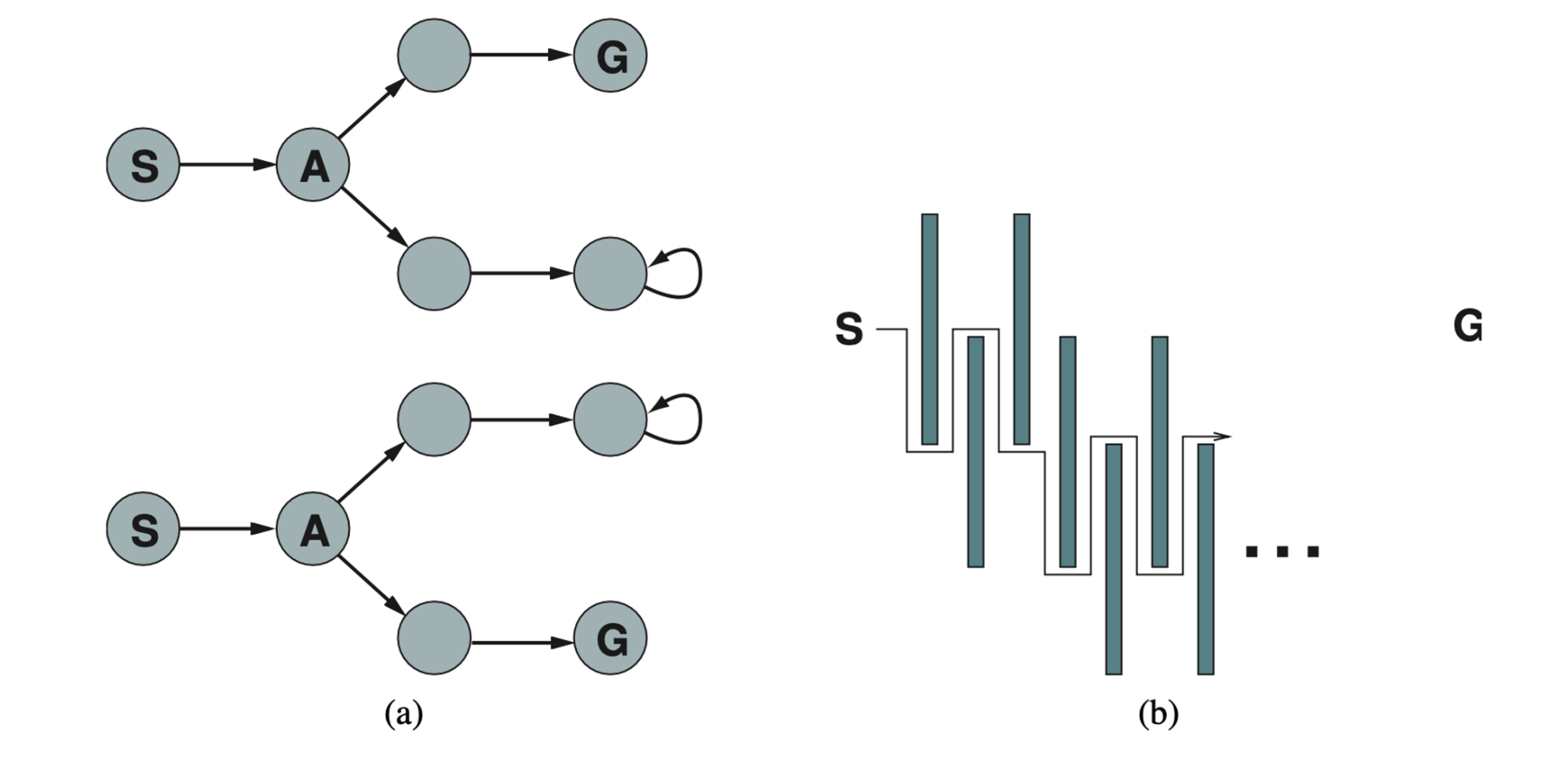
AND-OR Search Trees

In a deterministic environment, the only branching is introduced by the agent’s own choices in each state: I can do this action or that action. These nodes are called OR nodes. In a nondeterministic environment, branching is also introduced by the environment’s choice of outcome for each action. These are called AND nodes.

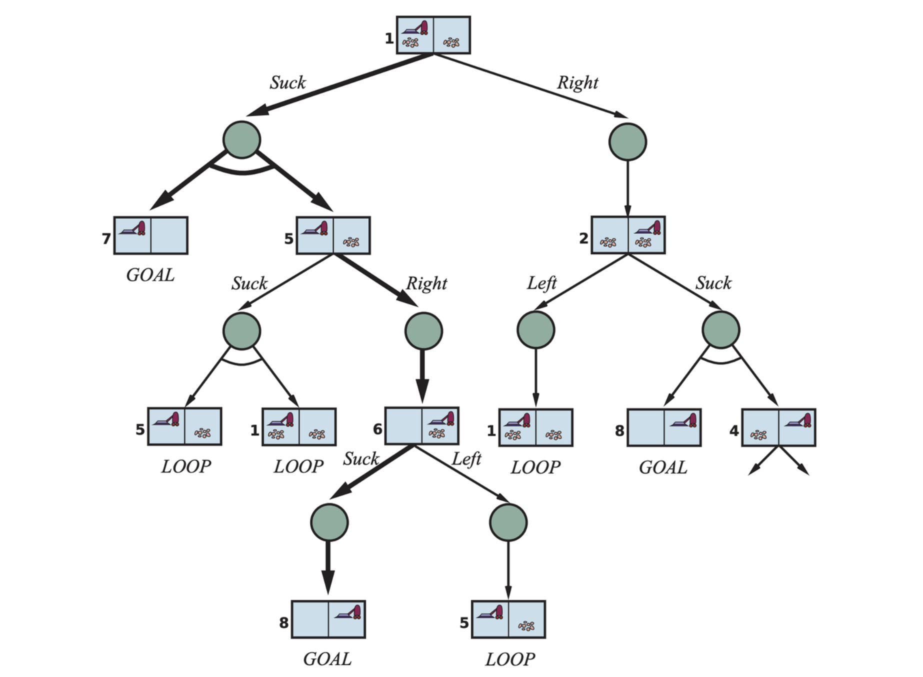
The first two levels of the search tree for the erratic vacuum world. State nodes are OR nodes where some action must be chosen. At the AND nodes, shown as circles, every outcome must be handled, as indicated by the arc linking the outgoing branches. The solution found is shown in bold lines.

A solution for an AND-OR search problem is a subtree of a complete search tree that

has a goal node at every leaf.
specifies one action at each of its OR nodes.
includes every outcome branch at each of its AND nodes.

// Depth-First Algorithm for AND-OR Graph Search
function AND_OR_Search(
    problem: Problem
): ConditionalPlan | Failure {
    return OR_Search(problem, problem.initial, [])
}

function OR_Search(
    problem: Problem, state: State, path: State[]
): ConditionalPlan | Failure {
    if (problem.isGoal(state)) return EmptyPlan
    if (IsCycle(state, path)) return Failure

    problem.actions(state).forEach(action => {
        const plan = AND_Search(
            problem,
            Results(state, action),
            [state, ...path]
        )
        if (plan !== Failure) return [action, ...plan]
    })

    return Failure
}

function AND_Search(
    problem: Problem, states: State[], path: State[]
): ConditionalPlan | Failure {
    const plan = {}
    for (let i = 0; i < states.length; ++i) {
        const state = states[i]
        const planI = OR_Search(problem, state, path)
        if (planI === Failure) return Failure

        plan[state] = planI
    }
    return plan
}

Search in Partially Observable Environments

In a partially observable environment, the agent’s percepts are not enough to pin down the exact state. That means that some of the agent’s actions will be aimed at reducing uncertainty about the current state.

Searching with no Observation

When the agent’s percepts provide no information at all, we have what is called a sensorless problem (or a conformant problem). Sometimes a sensorless plan is better even when a conditional plan with sensing is available.

The solution to a sensorless problem is a sequence of actions, not a conditional plan. But we search in the space of belief states rather than physical states. In belief-state space, the problem is fully observable because the agent always knows its own belief state.

The belief-state problem has the following components:

States: The belief-state space contains every possible subset of the physical states. If \(P\) has \(N\) states, then the belief-state problem has \(2^N\) belief state.
Initial state: Typically the belief state consisting of all states in \(P\).
Actions: Suppose the agent is in belief state \(b = \{ s_1, s_2\}\), but \(\text{ACTIONS}_P(s_1) \neq \text{ACTIONS}_P(s_2)\); then the agent is unsure of which actions are legal. If we assume that illegal actions have no effect on the environment, then it is safe to take the union of all the actions in any of the physical states in the current belief state \(b\):

\[ \text{ACTIONS}(b) = \bigcup_{s \in b} \text{ACTIONS}_P(s) \]

On the other hand, if an illegal action might lead to catastrophe, it is safer to allow only the intersection, that is, the set of actions legal in all the states.
Transition model: For deterministic actions, the new belief state has one result state for each of the current possible states:

\[ b' = \text{RESULT}(b, a) = \{s': s' = \text{RESULT}_P(s, a) \text{and} s\in b\} \]

With nondeterminism, the new belief state consists of all the possible results of appliying the action to any of the states in the current belief state:

\[ \begin{align} b' = \text{RESULT}(b, a) &= \{s': s' = \text{RESULT}_P(s, a) \text{and} s\in b\} \\ &= \bigcup_{s in b} \text{RESULT}_P(s, a) \end{align} \]

The size of \(b'\) will be the same or smaller than \(b\) for deterministic actions, but may be larger than \(b\) with nondeterministic actions.
Goal test: The agent necessarily achieves the goal if every state satisfies \(\text{IS-GOAL}_P(s)\). We aim to necessarily achieven the goal.
Action cost: If the same action can have different costs in different states, then the cost of taking an action in a given belief state could be one of serveral values.

Searching in Partially Observable Environments

Many problems cannot be solved without sensing. For a partially observable problem, the problem specification will specify a \(\text{PERCEPT}(s)\) function that resturns the percept received by the agent in a given state. If sensing is non-deterministic, then we can use a \(\text{PERCEPTS}\) function that returns a set of possible percepts.

The transition model between belief states for partially observable problems can be thought as occuring in three states.

The prediction stage computes the belief state resulting from the action, \(\hat{b} = \text{RESULT}(b, a)\).
The possible percepts stage computes the set of percepts that could be observed in the predicted belief state:

\[ \text{POSSIBLE-PERCEPTS}(\hat{b}) = \{o: o = \text{PERCEPT}(s) \text{ and } s \in \hat{b}\} \]
The update stage computes, for each possible percept, the belief state that would result from the percept. The updated belief state \(b_o\) is the set of states in \(\hat{b}\) that could have produced the percept:

\[ b_o = \text{UPDATE}(\hat{b}, o) = \{s: o = \text{PERCEPT}(s)\text{ and } s \in \hat{b}\} \]

Putting these three stages together, we obtain the possible belief state resulting from a given action and the subsequent possible percepts:

\[ \text{RESULTS}(b, a) = \{b_o: b_o = \text{UPDATE}(\text{PREDICT(b, a)}, o) \text{ and } o \in \text{POSSIBLE-PERCEPTS}(\text{PREDICT}(b, a))\} \]

Solving Partially Observable Problems

The AND-OR search algorithm can be applied directly to derive a solution.

Online Search Agents and Unknown Environments

So far we have concentrated on agents that use offline search algorithms. They compute a complete solution before taking their first action. In contract, an online search agent interleaves computation and action: first it takes an action, then it observes the environment and computes the next action.

Online Search Problems

An online search problem is solved by interleaving computation, sensing and acting. Assuming the environment is fully observable and stipulate that the agent knows only the following:

\(\text{ACTIONS}(s)\), the legal actions in state \(s\).
\(c(s, a, s')\), the cost of applying action \(a\) in state \(s\) to arrive at state \(s'\). Note that this cannot be used until the agent knows that \(s'\) is the outocme.
\(\text{IS-GOAL}(s)\), the goal test.

It is common to compare the cost that the agent incurs as it travels with the path cost the agent would incur if it knew the search space in advance —— that is, the optimal path in the known environment. In the language of online algorithms, this comparison is called the competitive ratio.

Online explorers are vulnerable to dead ends: states from which no goal state is reachable. In general, no algorithm can avoid dead ends in all state spaces.