Solving Problems by Searching

When the correct action to take is not immediately obvious, an agent may need to plan ahead: to consider a sequence of actions that form a path to a goal state. Such an agent is called a problem-solving agent, and the computational process it undertakes is called search.

Problem-Solving Agents

If the environment is completely unknown, then the agent can do no better than to execute one of the actions at random. With access to information about the world, the agent can follow the four-phase problem-solving process:

• Goal formulation: Goals organize behavior by limiting the objectives and hence the actions to be considered.
• Problem formulation: The agent devises a description of the states and actions necessary to reach the goal —— an abstract model of the relevant part of the world.
• Search: The agent simulates sequences of actions in its model, searching until it finds a sequence of actions that reaches the goal. Such a sequence si called a solution.
• Execution: The agent can now execute the actions in the solution, one at a time.

In a fully observable, deterministic, known environment, the solution to any problem is a fixed sequence of actions. This is an open-loop system: ignoring the percepts breaks the loop between agent and environment. If there is a chance that the model is incorrect, or the environment is nondeterministic, then the agent would be safer using a closed-loop approach that monitors the percepts.

Search Problems and Solutions

A search problem can be defined formally as follows:

• state space: A set of possible states that the environment can be in.
• initial state: that the agent starts in.
• A set of one or more goal states.
• The actions available to the agent. Given a state \(s\), \(\text{ACTIONS}(s)\) returns a finite set of actions that can be executed in \(s\). We say that each of these actions is applicable in \(s\).
• A transition model, which describes what each action does. \(\text{RESULT}(s, a)\) returns the state that results from doing action \(a\) in state \(s\).
• An action cost function, denoted by \(\text{ACTION-COST}(s, a, s')\), that gives the numeric cost of applying action \(a\) in state \(s\) to reach \(s'\).

A sequence of actions forms a path, and a solution is a path from the initial state to a goal state. An optimal solution has the lowest path cost among all solutions.

Formulating Problems

Formulating problems is a process of finding an appropriate level of abstraction. The abstraction is valid if we can elaborate any abstract solution into a solution in the more detailed world. The abstraction is useful if carrying out each of the actions in the solution is easier than the original problem.

Search Algorithms

A search algorithm takes a search problem as input and returns a solution, or an indication of failure. One type of algorithms superimposes a search tree over the state space graph, forming various paths from the initial state, trying to find a path that reaches a goal state.

Each node in the search tree corresponds to a state in the state space and the edges in the search tree correspond to actions. The root of the three corresponds to the initial state of the problem.

Best-first Search

A general approach for expand the frontier is called best-first search, in which a node \(n\) is chosen, with minimum value of some evaluation function, \(f(n)\).

// Best-first Search Algorithm
function BestFirstSearch(
    problem: Problem, f: EvaluateFunction
): Solution | Failure {
    let node = new Node({ state: problem.initial })
    const frontier = PriorityQueue<Node>({ orderBy: f })
    const reached = { [problem.initial]: node }

    while(!frontier.isEmpty()) {
        node = frontier.pop()
        if (problem.isGoal(node.state)) return node

        const children = Expand(problem, node)
        children.forEach(child => {
            const s = child.state
            if (!reached[s] || child.pathCost < reached[s].pathCost) {
                reached[s] = child
                frontier.push(child)
            }
        })
    }

    return Failure
}

function Expand(problem: Problem, node: Node): Node[] {
    const s = node.state
    return problem.actions(s).map(action => {
        const sp = problem.result(s.action)
        const cost = node.pathCost + problem.actionCost(s, action, sp)
        return new Node({
            state: s,
            parent: node,
            action: action,
            pathCost: cost,
        })
    })
}

💡 By employing different \(f(n)\) functions, we get different specific algorithms.

Search Data Structures

Node

A node in the tree is represented by a data structure with four components:

• node.STATE: the state to which the node corresponds
• node.PARENT: the node in the tree that generated this node
• node.ACTION: the action that was applied to the parent’s state to generate this node
• node.PATH-COST: the total cost of the path from the initial state to this node.

Following the PARENT pointers back from a node allows to recover the states and actions along the path to that node.

Frontier

A data structure is needed to store the frontier. The appropriate choice is a queue of some kind.

• IS-EMPTY(frontier): returns true only if there are no nodes in the frontier
• POP(frontier): removes the top node from the frontier and returns it
• TOP(frontier): returns (but does not remove) the top node of the frontier
• ADD(node, frontier): inserts node into its proper place in the queue

Three kinds of queues are used in search algorithms

• A priority queue first pops the node with the minimum cost according to some evaluation function, \(f\). It is used in best-first search.
• A FIFO queue first pops the node that was added to the queue first. It is used in breadth-first search.
• A LIFO queue pops first the most recently added node. It is used in depth-frist search.

Measuring Problem-Solving Performance

An algorithm’s performance can be evaluated in four ways:

• Completeness: Is the algorithm guaranteed to find a solution when there is one, and to correctly report failure when there is not?
• Cost optimality: Does it find a solution with the lowest path cost of all solutions?
• Time complexity: How long does it take to find a solution?
• Space complexity: How much memory is needed to perform the search?

For an implicit state space, complexity can be measured in terms of \(d\), the depth or number of actions in an optimal solution; \(m\), the maximum number of actions in any path; and \(b\), the branching factor or number of successors of a node that need to be considered.

Uninformed Search Strategies

An uninformed search algorithm is given no clue about how close a state is to the goBal(s).

Breadth-First Search

When all actions have the same cost, an appropriate strategy is breadth-first-search, in which the root node is expanded first, then all the successors of the root node are expanded next, then their successors, and so on.

// Breadth-First Search
function BreathFirstSearch(problem: Problem): Node | Failure {
    const node = new Node(problem.initial)
    
    if (problem.isGoal(node.state)) return node

    const frontier = FIFOQueue<Node>()
    const reached = new Set()

    frontier.push(node)
    reached.add(problem.initial)

    while (!frontier.isEmpty()) {
        const node = frontier.pop()
        const children = Expand(problem, node)
        children.forEach(child => {
            const s = child.state
            if (problem.isGoal(s)) return child
            if (!reached.has(s)) {
                reached.add(s)
                frontier.push(child)
            }
        })
    }

    return Failure
}

// Uniform Cost Search
function UniformCostSearch(problem: Problem): Node | Failture {
    return BestFirstSearch(problem, PathCost)
}

Suppose a uniform tree where every state has \(b\) successors, the total number of nodes generated is

\[ 1 + b + b^2 + \cdots + b^d = O(b^d) \]

All the nodes remain in memory, so both time and space complexity are \(O(b^d)\).

💡 In general, exponential-complexity search problems cannot be solved by uninformed search for any but the smallest instances.

Dijkstra’s Algorithm or Uniform-Cost Search

When actions have different costs, an obvious choice is to use best-first search where the evaluation function is the cost of the path from the root to the current node. This is called Dijkstra’s algorithm or uniform-cost search by the AI community.

Given the cost of the optimal solution \(C^*\) and \(\epsilon\), a lower bound on the cost of each action, then the algorithm’s worst-case time and space complexity is \(O(b^{1 + \lfloor C^* / \epsilon \rfloor})\), which can be much bettwen than \(b^d\). This is because uniform-cost search can explore large trees of actions with low costs before exploring paths involving a high-cost and perhaps useful action.

Depth-First Search and the Problem of Memory

Depth-first search always expands the deepest node in the frontier first. It could be implemented as a call to BEST-FIRST-SEARCH where the evaluation function \(f\) is the negative of the depth.

In infinite state spaces, depth-first search is not systematic: it can get stuck going down an infinite path, even if there are no cycles.

But where a tree-like search is feasible, depth-first search has much smaller needs for memory. A reached table is no kept at all, and the frontier is very small. A memory complexity of a depth-first tree-like search is \(O(bm)\), where \(b\) is the branching factor and \(m\) is the maximum depth of the tree.

💡 Because of its parsimonious use of memory, depth-first tree-like search has been adopted as the basic workhorse of many areas of AI.

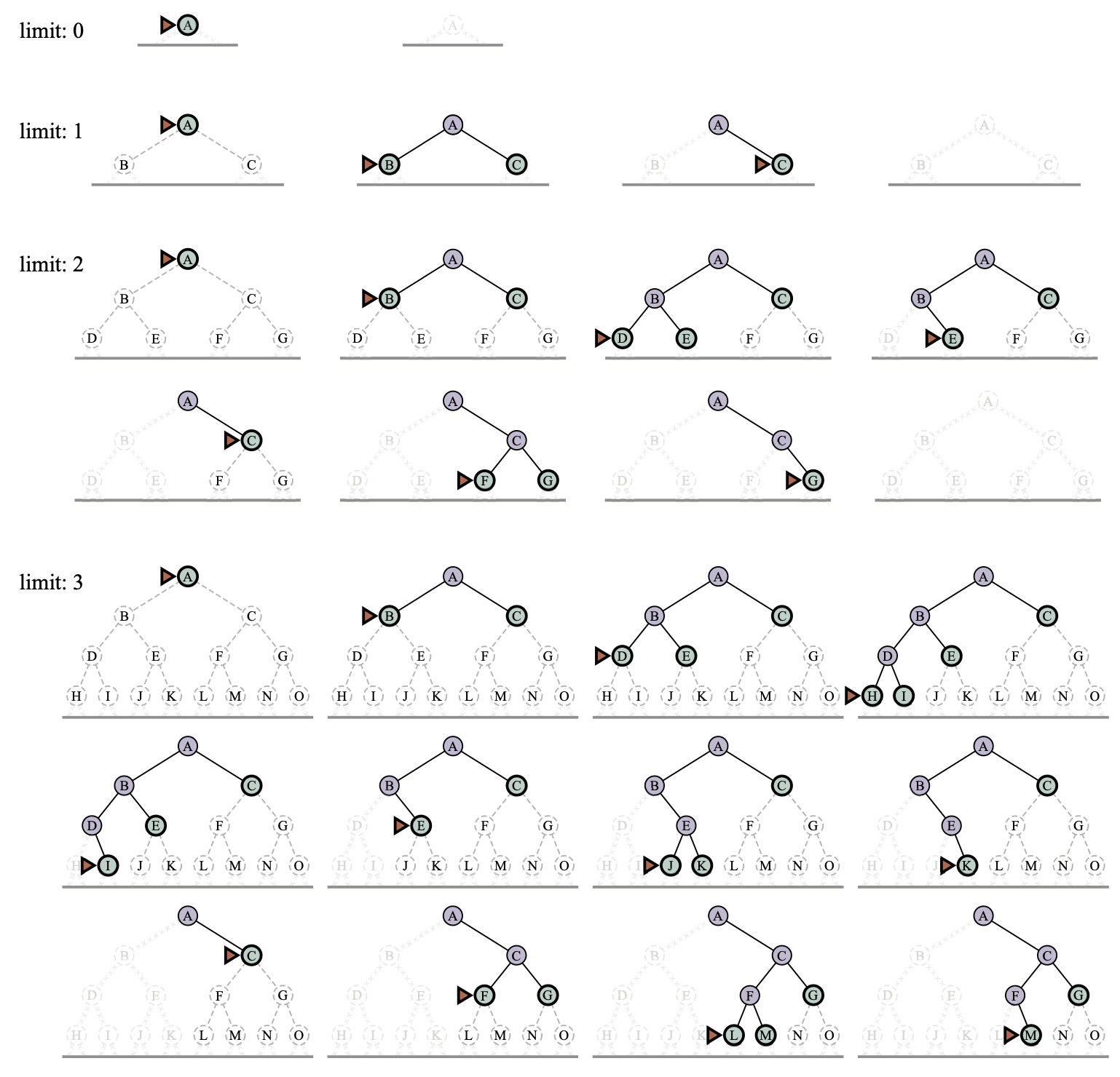
Depth-Limited and Iterative Deepening Search

To keep depth-first search from wandering down and infinite path, we can use depth-limited search, a version of depth-first search in which we supply a depth limit, \(l\), and treat all nodes in depth \(l\) as if they had no successors. The time complexity is \(O(b^l)\) and the space complexity is \(O(bl)\).

Iterative deepening search solves the problem of picking a good value for \(l\) by trying all values: first 0, then 1, then 2 and so on —— until either a solution is found, or the depth limited search returns the failure value rather than the cutoff value.

// Iterative Deepening Search
function IterativeDeepeningSearch(problem: Problem): Node | Failure {
    let depth = 0
    while (true) {
        const result = DepthLimitedSearch(problem, depth)
        if (result != CUTOFF) return result
    }
}

function DepthLimitedSearch(problem: Problem, limit: number): Node | Failure {
    const frontier = LIFOQueue<Node>()
    const result = Failure

    frontier.push(problem.initial)

    while (!frontier.isEmpty()) {
        const node = frontier.pop()
        if (problem.isGoal(node.state)) return node
        if (Depth.node > limit) {
            result = CUTOFF
        } else if (!IsCycle(node)) {
            Expand(problem, node).forEach(child => {
                frontier.push(child)
            })
        }
    }

    return result
}

Four iterations of iterative deepening search for goal M on a binary tree, with the depth limit varying from 0 to 3. Note the interior nodes form a single path. The triangle marks the node to expand next; green nodes with dark outlines are on the frontier; the very faint nodes probably can’t be part of a solution with this depth limit.

💡 In general, iterative deepening is the preferred uninformed search method when the search state space is larger than can fit in memory and the depth of the solution is not known.

Bidirectional Search

Bidirectional search simultaneously searches forward from the initial state and backwards from the goal state(s), hoping that the two searches will meet. The motivation is that \(b^{d/2} + b^{d/2}\) is much less than \(b^d\).

// Bidirectional Best-First Search
function BIBF_Search(
    problemF: Problem,    // forward problem
    fF: EvaluateFunction, // evaluate function for forward problem
    problemB: Problem,    // backward problem
    fB: EvaluateFunction, // evaluate function for backward problem
): Node | Failure {
    const nodeF = new Node(problemF.initial)
    const nodeB = new Node(problemB.initial)
    const frontierF = PriorityQueue<Node>()
    const frontierB = PriorityQueue<Node>()
    const reachedF = { [nodeF.state]: nodeF }
    const reachedB = { [nodeB.state]: nodeB }

    frontierF.push(nodeF)
    frontierB.push(nodeB)

    let solution = Failure

    while (!Terminated(solution, frontierF, frontierB)) {
        if (fF(frontierF.top()) < fB(frontierB.top())) {
            solution = Proceed(
                FORWARD, prblemF, frontierF, reachedF,
                reachedB, solution)
        } else {
            solution = Proceed(
                BACKWARD, prblemB, frontierB, reachedB,
                reachedF, solution)

        }
    }

    return solution
}

function Proceed(
    dir: FORWARD | BACKWARD,
    problem: Problem,
    frontier, reached, reached2, solution
): Solution {
    const node = frontier.pop()
    Expand(problem, node).forEach(child => {
        const s = child.state
        if (!reached[s] || PathCost(child) < PathCost(reached[s])) {
            reached[s] = child
            frontier.push(child)
            if (reached2[s]) {
                solution2 = JoinNodes(dir, child, reached2[s])
                if (PathCost(solution2) < PathCost(solution)) {
                    solution = solution2
                }
            }
        }
    })

    return solution
}

For this to work, we need to keep track of two frontiers and two tables of reached states, and we need to be able to reason backwards: if state \(s'\) is a successor of \(s\) in the forward direction, then we need to know that \(s\) is a successor of \(s'\) in the backward direction.

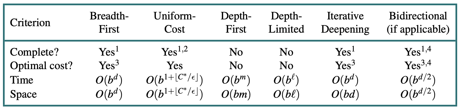
Comparing Uninformed Search Algorithms

Evaluation of search algorithms. b is the branching factor; m is the maximum depth of the search tree; d is the depth of the shallowest solution, or is m when there is no solution; l is the depth limit. Superscript caveats are as follows: 1 complete if b is finite, and the state space either has a solution or is finite. 2 complete if all action costs are ≥ ε > 0; 3 cost-optimal if action costs are all identical; 4 if both directions are breadth-first or uniform-cost.

Informed(Heuristic) Search Strategies

Informed Search strategy —— one that uses domain-specific hints about the location of goals —— can find solutions more efficiently than an uninformed strategy. This hints come in the form of a heuristic function, denoted \(h(n)\):

\[ h(n) = \small \text{estimated cost of the cheapest path from the state at node } n \text{ to a goal state} \]

Greedy Best-First Search

Greedy best-first search is a form of best-first search that expands first the node with the lowest \(h(n)\) value —— the node that appears to be closest to the goal. So the evaluation function \(f(n) = h(n)\).

A* Search

A* search uses the evaluation function

\[ f(n) = g(n) + h(n) \]

where \(g(n)\) is the path cost from the initial state to node \(n\), and \(h(n)\) is the estimated cost of the shortest path from \(n\) to a goal state, so we have

\[ f(n) = \small \text{estimated cost of the best path that continues from } n \text{ to a goal.} \]

An example of A* search is shown as below.

Stages in an A* search for Bucharest. Notes are labeled with f = g + h. The h values are the straight-line distances to Bucharest.

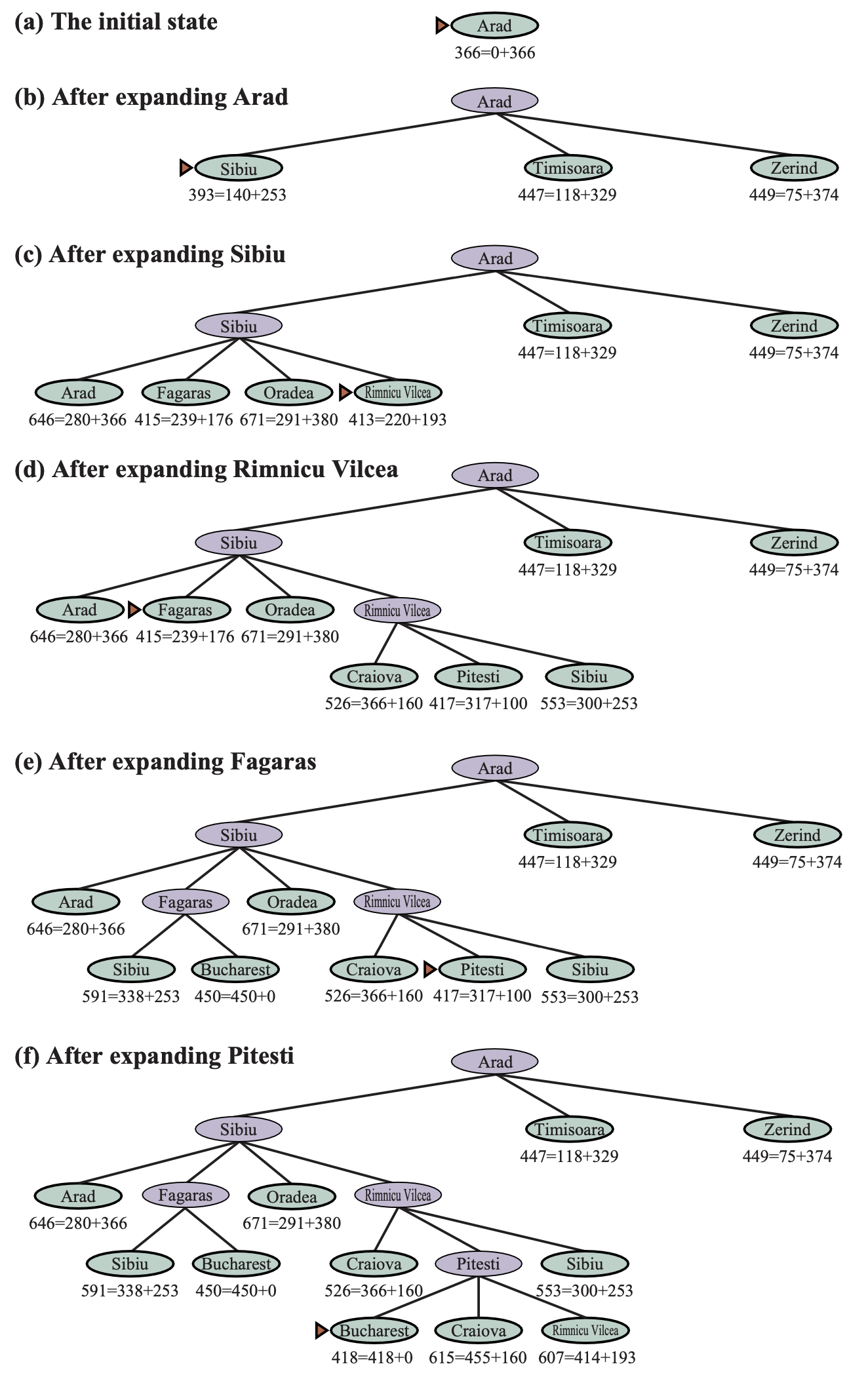
Stages in an A* search for Bucharest. Notes are labeled with f = g + h. The h values are the straight-line distances to Bucharest.

Whether A* is cost-optimal depends on certain properties of the heuristic. A key property is admissibility: an admissible heuristic is one that never overestimates the cost to reach a goal.

A slightly stronger property is called consistency. A heuristic \(h(n)\) is consistent if, for every node \(n\) and every successor \(n'\) of \(n\) generated by an action \(a\), we have

\[ h(n) \leq c(n, a, n') + h(n') \]

This is a form of the triangle inequality. If the heuristic \(h\) is consistent, then the single number \(h(n)\) will be less than the sum of the cost \(c(n, a, a')\) of the action from \(n\) to \(n'\) plus the heuristic estimate \(h(n')\).

💡 Every consistent heuristic is admissible (but not vice versa), so with a consistent heuristic, A* is cost-optimal. In addition, with a consistent heuristic, the first time we reach a state it will be on an optimal path, so we never have to re-add a state to the frontier, and never have to change an entry in reached.

Search Contours

A useful way to visualize a search is to draw contours in the state space. Inside the contour labeled \(c\), all nodes have \(f(n) = g(n) + h(n) \leq c\). With uninform-cost search, the contours will be “circular” around the start state, spreading out equally in all directions with no preference towards the goal. With A* search using a good heuristic, the \(g+h\) bands will stretch toward a goal state and become more narrowly focused around an optimal path.

If \(C^*\) is the cost of the optimal solution path, then we can say the following:

• A* expands all nodes that can be reached from the initial state on a path where every node on the path has \(f(n) < C^*\). We say these are surely expanded nodes.
• A* might then expand some of the nodes right on the “goal contour” (where \(f(n) = C^*\)) before selecting a goal node.
• A* expands no nodes with \(f(n) > C^*\).

We say that A* with a consistent heuristic is optimally efficient in the sense that any algorithm that extends search paths from the initial state, and uses the same heuristic information, must expand all nodes that are surely expanded by A*.

💡 That A* search is complete, cost-optimal, and optimally efficient among all such algorithms is rather satisfying. Unfortunately, it does not mean that A* is the answer to all our searching needs. The catch is that for many problems, the number of nodes expanded can be exponential in the length of the solution.

Satisficing Search: Inadmissible Heuristic and Weighted A*

A* search has many good qualities, but it expands a lot of nodes. We can explore fewer nodes (taking less time and space) if we are willing to accept solutions that are suboptimal, but are “good enough” —— what are called satisficing solutions. If we allow A* search to use an inadmissible heuristic —— one that may overestimate —— then we risk missing the optimal solution, but the heuristic can potentially be more accurate, thereby reducing the number of nodes expanded.

Two searches on the same grid: (a) an A∗ search and (b) a weighted A∗ search with weight W = 2. The gray bars are obstacles, the purple line is the path from the green start to red goal, and the small dots are states that were reached by each search. On this particular problem, weighted A∗ explores 7 times fewer states and finds a path that is 5% more costly.

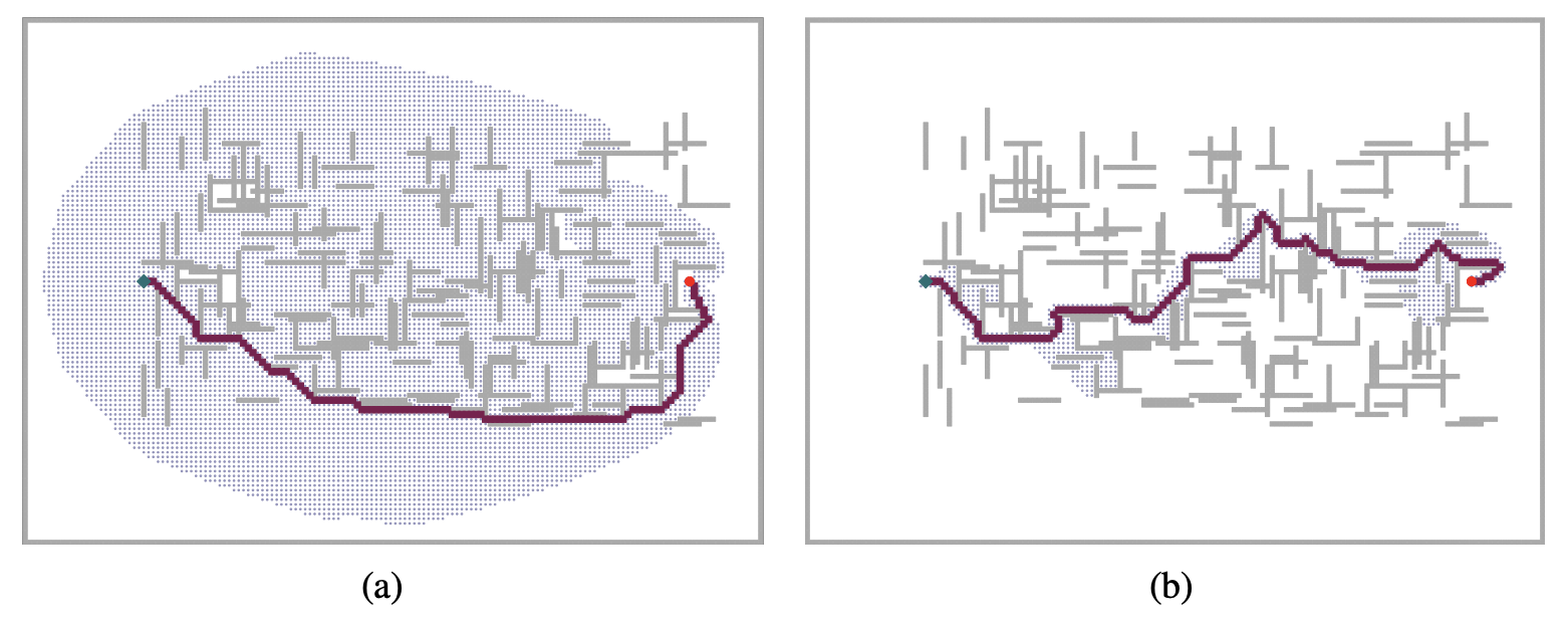
Two searches on the same grid: (a) an A∗ search and (b) a weighted A∗ search with weight W = 2. The gray bars are obstacles, the purple line is the path from the green start to red goal, and the small dots are states that were reached by each search. On this particular problem, weighted A∗ explores 7 times fewer states and finds a path that is 5% more costly.

With an approach called weighted A* search where we weight the heuristic value more heavily, giving us the evaluation function \(f(n) = g(n) + W \times h(n)\), for some \(W > 1\).

In general, if the optimal solution costs \(C^*\), a weighted A* search will find a solution that costs somewhere between \(C^*\) and \(W \times C^*\); but in practice we usually get results much closer to \(C^*\) than \(W \times C^*\).

Searches can be considered that evaluates states by combining \(g\) and \(h\) in various ways.

\[ \begin{aligned} \text{A* search}: &\ \ \ \ \ g(n) + h(n) & (W = 1) \\ \text{Uniform-cost search}: &\ \ \ \ \ g(n) & (W = 0) \\ \text{Greedy best-first search}: &\ \ \ \ \ h(n) & (W = \infty) \\ \text{Weighted A* search}: &\ \ \ \ \ g(n) + W \times h(n) & (1 < W < \infty) \\ \end{aligned} \]

There are a variety of suboptimal search algorithms, which can be characterized by the criteria for what counts as “good enough”.

• bounded suboptimal search: we look for a solution that is guaranteed to be within a constant factor \(W\) of the optimal cost.
• bounded-cost search: we look for a solution whose cost is less than some constant \(C\).
• unbounded-cost search: we accept a solution of any cost, as long as we can find it quickly.

Memory-Bounded Search

Memory is split between the frontier and the reached states.

Beam search limits the size of the frontier. The easiest approach is to keep only the \(k\) nodes with the best \(f\)-scores, discarding any other expanded nodes.

**Iterative-deepening A* search (IDA*)** is to A* what iterative-deepening search is to depth-first: IDA* gives us the benefits of A* without the requirement to keep all reached states in memory, at a cost of visiting some states multiple times. In IDA* the cutoff is the \(f\)-cost \((g + h)\); at each iteration, the cutoff value is the smallest \(f\)-cost of any node that exceeded the cutoff on the previous iteration.

Recursive best-first search (RBFS) attempts to mimic the operation of standard best-first search, but using only linear space.

Bidirectional Heuristic Search

Bidirectional search is sometimes more efficient than unidirectional search, sometimes not. In general, if we have a very good heuristic, then A* search produces search contours that are focused on the goal, and adding bidirectional search does not help much.

Heuristic Functions

The Effect of Heuristic Accuracy on Performance

One way to characterize the quality of a heuristic is the effective branching factor \(b^*\). If the total number of nodes generated by A* for a particular problem is \(N\) and the solution depth is \(d\), then \(b^*\) is the branching factor that a uniform tree of depth \(d\) would have to have in order to contain \(N+1\) nodes. Thus

\[ N + 1 = 1 + b^* + (b^*)^2 + \cdots + (b^*)^d \]

💡 The effective branching factor can vary across problem instances, but usually for a specific domain it is fairly constant across all nontrivial problem instances. Therefore, experimental measurements of \(b^*\) on a small set of problems can provide a good guide to the heuristic’s overall usefulness.

Generating Heuristic from Relaxed Problems

A problem with fewer restrictions on the actions is called a relaxed problem. The state-space graph of the relaxed problem is a supergraph of the original state space because the removal of restrictions creates added edges in the graph. Because the relaxed problem adds edges to the state-space graph, any optimal solution in this original problem is, by definition, also a solution in the relaxed problem; but the relaxed problem may have better solutions if the added edges provide shortcuts. Hence, the cost of an optimal solution to a relaxed problem is an admissible heuristic for the original problem.

For example, if the 8-puzzle actions are described as

A tile can move from square X to square Y if X is adjacent to Y and Y is blank.

we can generate three relaxed problems by removing one or both of the conditions:

1. A tile can move from square X to square Y if X is adjacent to Y.

2. A tile can move from square X to square Y if Y is blank.

3. A tile can move from square X to square Y.

From (a), we can derive Manhattan distance as a heuristic function. From (c), we can derive direct distance as a heuristic function.

If a collection of admissible heuristic \(h_1, h_2, \dots, h_m\) is available for a problem and none of them is clearly better than others, which should be choose? As it turns out, we can have the best of all worlds, by defining

\[ h(n) = \max\{h_1(n), h_2(n), \dots, h_k(n)\} \]

This composite heuristic picks whichever function is most accurate on the node in question. Because the \(h_i\) components are admissible, \(h\) is admissible (and if \(h_i\) are all consistent, \(h\) is consistent). Furthermore, \(h\) dominates all of its component heuristics.

Generating Heuristics from Subproblems: Pattern Databases

Admissible heuristics can also be derived from the solution cost of a subproblem of a given problem.

Generating Heuristics with Landmarks

A perfect heuristic could be generated by precomputing and storing the cost of the optimal path between landmark points from the vertices. For each landmark \(L\) and for each other vertex \(v\) in the graph, we compute and store \(C^*(v, L)\), the exact cost of the optimal path from \(v\) to \(L\). Given the stored \(C^*\) tables, we can easily create an efficient heuristic: the minimum, over all landmarks, of the cost of getting from the current node to the landmark, and then to the goal:

\[ h_L(n) = \min_{L \in \text{Landmarks}} C^*(n, L) + C^*(L, goal) \]

\(h_L(n)\) is efficient but not admissible.

\[ h_{DH}(n) = \max_{L \in \text{Landmarks}} \big|C^*(n, L) - C^*(goal, L)\big| \]

This is called a differential heuristic.

Summary

• Before an agent can start searching, a well-defined problem must be formulated.
• A problem consists of five parts: the initial state, a set of actions, a transition model describing the results of those actions, a set of goal states, and an action cost function.
• The environment of the problem is represented by a state space graph. A path through the state space (a sequence of actions) from the initial state to a goal state is a solution.
• Search algorithms generally treat states and actions as atomic, without any internal structure (although we introduced features of states when it came time to do learning).
• Search algorithms are judged on the basis of completeness, cost optimality, time complexity, and space complexity.
• Uninformed search methods have access only to the problem definition. Algorithms build a search tree in an attempt to find a solution. Algorithms differ based on which node they expand first:
  • Best-first search selects nodes for expansion using an evaluation function.
  • Breadth-first search expands the shallowest nodes first; it is complete, optimal for unit action costs, but has exponential space complexity.
  • Uniform-cost search expands the node with lowest path cost, \(g(n)\), and is optimal for general action costs.
  • Depth-first search expands the deepest unexpanded node first. It is neither complete nor optimal, but has linear space complexity. Depth-limited search adds a depth bound.
  • Iterative deepening search calls depth-first search with increasing depth limits until a goal is found. It is complete when full cycle checking is done, optimal for unit action costs, has time complexity comparable to breadth-first search, and has linear space complexity.
  • Bidirectional search expands two frontiers, one around the initial state and one around the goal, stopping when the two frontiers meet.
• Informed search methods have access to a heuristic function \(h(n)\) that estimates the cost of a solution from \(n\). They may have access to additional information such as pattern databases with solution costs.
  • Greedy best-first search expands nodes with minimal \(h(n)\). It is not optimal but is often efficient.
  • A∗ search expands nodes with minimal \(f (n) = g(n) + h(n)\). A∗ is complete and optimal, provided that \(h(n)\) is admissible. The space complexity of A∗ is still an issue for many problems.
  • Bidirectional A∗ search is sometimes more efficient than A∗ itself.
  • IDA∗ (iterative deepening A∗ search) is an iterative deepening version of A∗, and thus adresses the space complexity issue.
  • RBFS (recursive best-first search) and SMA∗ (simplified memory-bounded A∗) are robust, optimal search algorithms that use limited amounts of memory; given enough time, they can solve problems for which A∗ runs out of memory.
  • Beam search puts a limit on the size of the frontier; that makes it incomplete and suboptimal, but it often finds reasonably good solutions and runs faster than complete searches.
  • Weighted A∗ search focuses the search towards a goal, expanding fewer nodes, but sacrificing optimality.
• The performance of heuristic search algorithms depends on the quality of the heuristic function. One can sometimes construct good heuristics by relaxing the problem definition, by storing precomputed solution costs for subproblems in a pattern database, by defining landmarks, or by learning from experience with the problem class.