Convexity-based Methods

Convex objects have certain properties that make them highly suitable for use in collision detection tests.

• The existence of a separating plane for nonintersecting convex objects.
• The distance between two points — one from each object — is at a local minimum. The distance is also a global minimum.

Concave objects do not share these characteristics.

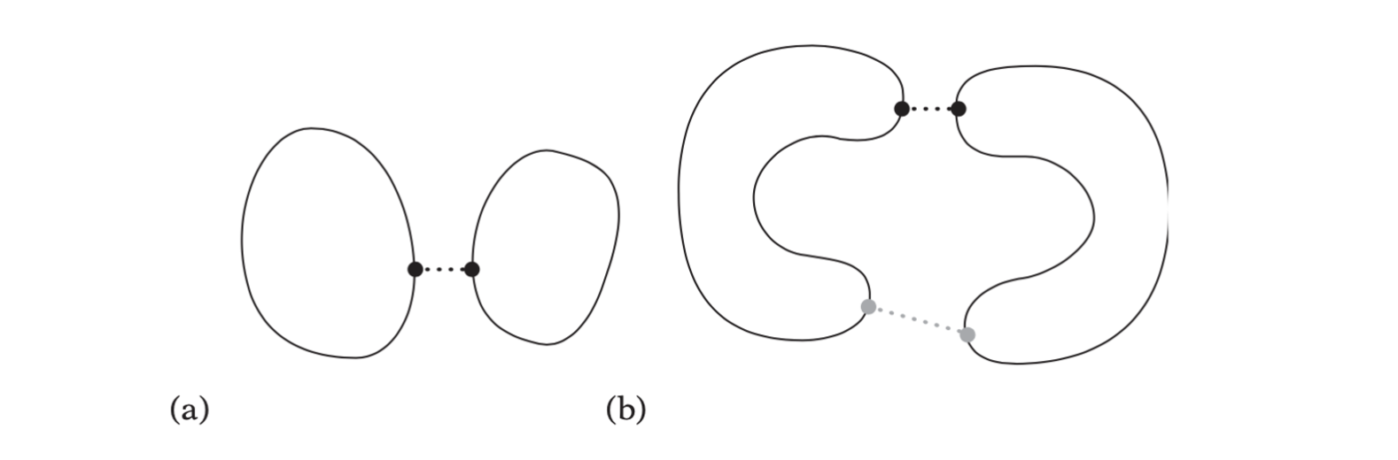
(a)For two convex objects a local minimum distance between two points is always a global minimum. (b) For two concave objects the local minimum distance between two points (in gray) is not necessarily a global minimum (in black).

(a)For two convex objects a local minimum distance between two points is always a global minimum. (b) For two concave objects the local minimum distance between two points (in gray) is not necessarily a global minimum (in black).

Boundary-based Collision Detection

Assuming the polyhedra are both in the same frame of reference (accomplished by, for example, transforming \(Q\) into the space of \(P\)), their intersection can be determined as follows.

1. Intersect each edge of \(P\) against polyhedron \(Q\). If an edge lies partly or fully inside \(Q\), stop and report the polyhedra as intersecting.
2. Conversely, intersect each edge of \(Q\) against polyhedron \(P\). If an edge lies partly or fully inside \(P\), stop and report \(P\) and \(Q\) as intersecting.
3. Finally, to deal with the degenerate case of identical objects (such as cubes) passing through each other with their faces aligned, test the centroid of each face of \(Q\) against all faces of \(P\). If a centroid is found contained in \(P\), stop and return intersection.
4. Return non-intersection.

For the first two steps, testing against edges are quite expensive, it can be changed to follows:

1. Test each vertex \(Q\) against all faces of \(P\). If any vertex is found to lie inside all faces of \(P\), stop and return the polyhedra as intersecting.
2. Repeat the previous step, but now testing each vertex of \(P\) against the faces of \(Q\).

Closest-features Algorithms

For polyhedra, rather than tracking the closest points and using the closest points of the previous frame as a starting point a better approach is to trach the closest features (vertices, edges, or faces) from frame to frame. A pair of features, one from each of the two disjoint polyhedra, are said to be the closest features if they contain a pair of closest points for the polyhedra.

The V-Clip Algorithm

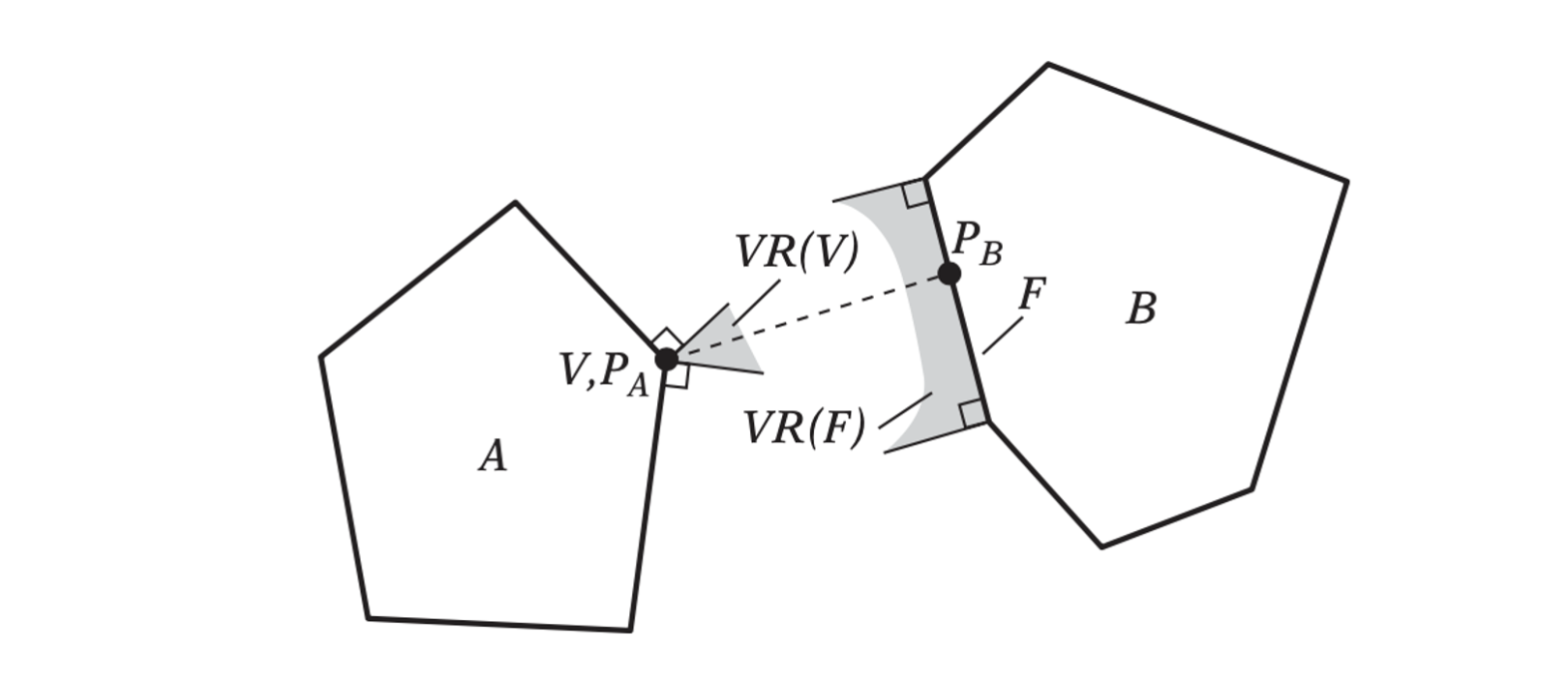
Two nonintersecting 2D polyhedra A and B. Indicated is the vertex-face feature pair V and F, constituting the closest pair of features and containing the closest pair of points, PA and PB, between the objects.

Two nonintersecting 2D polyhedra A and B. Indicated is the vertex-face feature pair V and F, constituting the closest pair of features and containing the closest pair of points, PA and PB, between the objects.

💡 Theorem: Let \(F_A\) and \(F_B\) be a pair of features from two disjoint convex polyhedra, \(A\) and \(B\), and let \(VR(F_A)\) and \(VR(F_B)\) denote their Voronoi regions. Let \(P_A \in F_A\) and \(P_B \in F_B\) be a pair of closest points between the features. Then, if \(P_A \in VR(F_B)\) and \(P_B \in VR(F_A)\), \(F_A\) and \(F_B\) are a globally closest pair of features and \(P_A\) and \(P_B\) are a globally closest pair of points between \(A\) and \(B\) (albeit not necessarily unique).

V-Clip starts with two features, one from each input polyhedron. At each iteration of the algorithm, the features are tested to see if they meet the conditions of the theorem for being a closest pair of features. If so, the algorithm terminates, returning a result of nonintersection along with the pair of closest features. If the conditions are not met, V-Clip updates one of the features to a neighboring feature, where the neighbors of a feature are defined as follows.

• The neighbors of a vertex are the edges incident to the vertex.
• The neighbors of a face are the edges bounding the face.
• The neighbors of an edge are the two vertices and the two faces incident to the edge.

Feature pair transition chart in which solid arrows indicate strict decrease of interfeature distance and dashed arrows indicate no change.

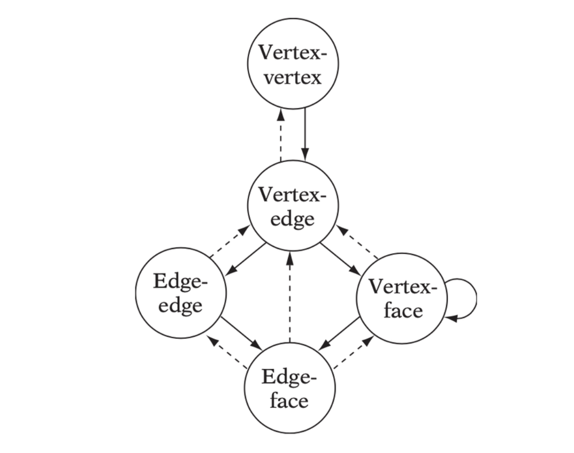
Feature pair transition chart in which solid arrows indicate strict decrease of interfeature distance and dashed arrows indicate no change.

Hierarchical Polyhedron Representations

Most well known of the nested polyhedron representations is the Dobkin-Kirkpatrick hierarchy. The Dobkin-Kirkpatrick hierarchy can be used for queries such as finding an extreme vertex in a given direction, locating the point on a polyhedron closest to a given point, or determining the intersection of two polyhedra.

The Dobkin-Kirkpatrick Hierarchy

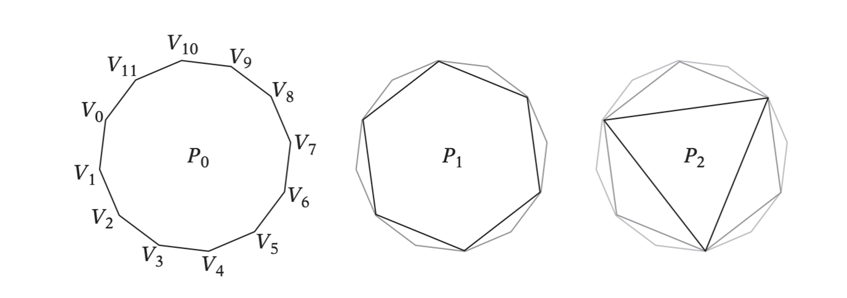
The Dobkin-Kirkpatrick (DK) hierarchy of a d-dimensional polyhedron \(P\) is a sequence \(P_0, P_1, \dots, P_k\) of nested increasingly smaller polytopal approximations of \(P\), where \(P = P_0\) and \(P_{i+1}\) is obtained from \(P_i\) by deletion of a subset of the vertices of \(P_i\). The subset of vertices is selected to form a maximal set of independent vertices (that is, such that no two vertices in the set are adjacent to each other). The construction of the hierarchy stops with the innermost polyhedron \(P_k\) being a d-simplex (a tetrahedron in 3D).

// Given a set s of vertices, compute a maximal set of independent vertices
Set IndependentSet(Set s) {
    // Initialize i to the empty set
    Set i = EmptySet();
    // Loop over all vertices in the input set
    for (all vertices v in s) {
        // If unmarked and has 8 or fewer neighboring vertices...
        if (!Marked(v) && Degree(v) <= 8) {
            // Add v to the independent set and mark all of v’s neighbors
            i.Add(v);
            s.MarkAllVerticesAdjacentToVertex(v);
        }
    }
    return i;
}

An example of constructing the DK hierarchy of a polygon.

The Dobkin–Kirkpatrick hierarchy of the convex polygon P = P0.

Given a DK hierarchy, many different queries can be answered in an efficient manner.

The supporting plane H, for (a) P2 and (b) P1, through the point on the polyhedron closest to a query point S.

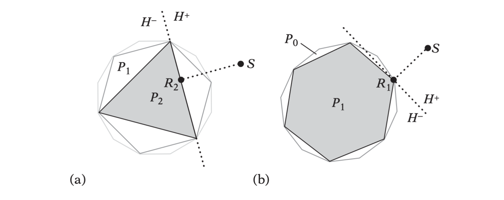
The supporting plane H, for (a) P2 and (b) P1, through the point on the poly- hedron closest to a query point S.

Starting at the innermost polyhedra \(P_i\), \(i = 2\), the closest point \(R_i\) on \(P_i\) to \(S\) is found through straightforward calculation. If \(R_i = S\), then \(S\) is contained in \(P\) and the algorithm stops. Otherwise, knowing \(R_i\), the closest point for \(P_{i-1}\) is found as follows. Let \(H\) be the supporting plane for \(P_i\) through \(R_i\). \(P_{i - 1}\) can now be described as consisting of the part in front of \(H\) and the part behind \(H\)

\[ P_{i-1} = (P_{i-1} \cap H^+)\cup(P_{i-1} \cap H^-) \]

• The closest point between \(P_{i-1} \cap H^-\) and \(S\) is directly given by \(R_i\).
• Since \(P_{i-1} \cap H^+\) is defined by one vertex and two edges, the closest point between \(P_{i-1} \cap H^+\) and \(S\) is computed in constant time.

Linear and Quadratic Programming

Collision detection problems can be expressed as linear and quadratic programming problems.

Linear Programming

The linear programming problem is the problem of optimizing (maximizing or minimizing) a linear function with respect to a finite set of linear constraints. The linear function to be optimized is called the objective function.

Without loss of generality, linear programming (LP) problems are here restricted to maximization of the objective function and to involve constraints of the form \(f(x_1, x_2, \dots, x_n) \leq c\) only.

A linear inequality of \(n\) variables geometrically defines a halfspace in \(\mathbb{R}^n\). The region of feasible solutions defined by a set of \(m\) inequalities therefore corresponds to a convex polyhedron \(P\), \(P = H_1 \cap H_2 \cap \cdots \cap H_m\). Note also that the objective function can be seen as a dot product between the vectors \(\textbf{x} = (x_1, x_2, \dots, x_n)\) and \(\textbf{c} = (c_1, c_2, \dots, c_n)\). The LP problem is therefore geometrically equivalent to that of finding a supporting point \(\textbf{x}\) of \(P\) in direction \(\textbf{c}\).

💡 The intersection problem can be expressed as an LP problem in the following way. Let the two polyhedra be given in terms of their vertices. Now a linear programming problem can be set up to determine whether there exist coefficients for a plane such that it forms a separating plane for the two polyhedra.

Fourier-Motzkin Elimination

It operates by successive rewrites of the system, eliminating one variable from the system on each rewrite. When only one variable is left, the system is trivially consistent if the largest lower bound for the variable is less than the smallest upper bound for the variable.

Seidel's Algorithm

A simple method for solving linear programming problems in \(d\) variables and \(m\) inequality constraints is Seidel’s algorithm. Seidel’s algorithm has an expected running time of \(O(d!m)\). Although the algorithm is not practical for large \(d\) it is quite efficient for small \(d\).

The two triangles A = (1,0), (5,−1), (4,3) and B = (0,0), (4,1), (1,4) defined as the intersection of three halfspaces each.

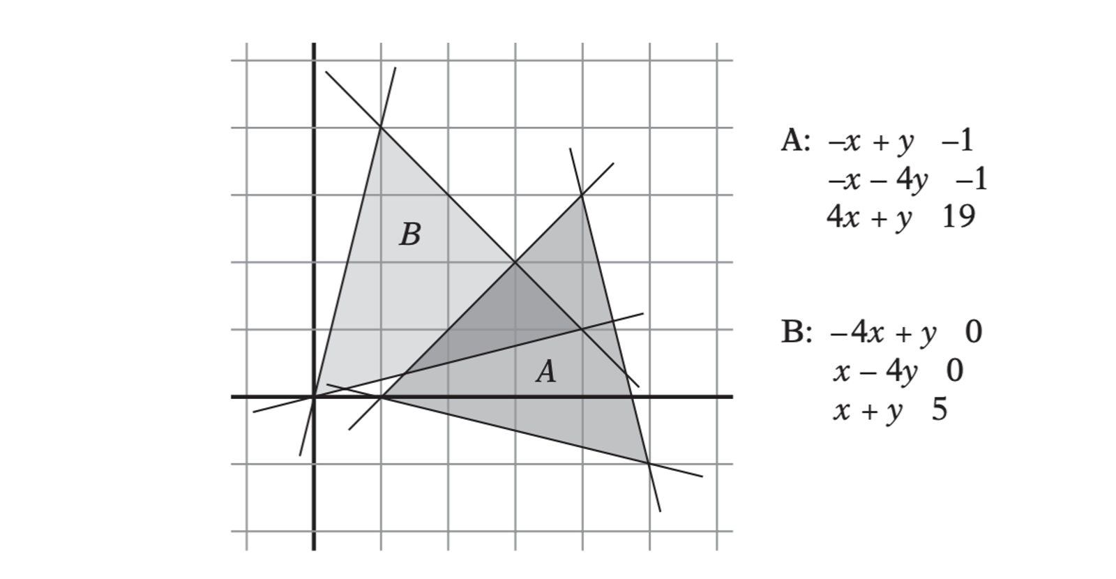
The two triangles A = (1,0), (5,−1), (4,3) and B = (0,0), (4,1), (1,4) defined as the intersection of three halfspaces each.

At top left, the six halfspaces from the two triangles given above. Remaining illustrations show Seidel’s algorithm applied to these six halfspaces. The feasible region is shown in light gray and the current halfspace is shown in thick black. Arrows indicate the 1D constraints in the recursive call.

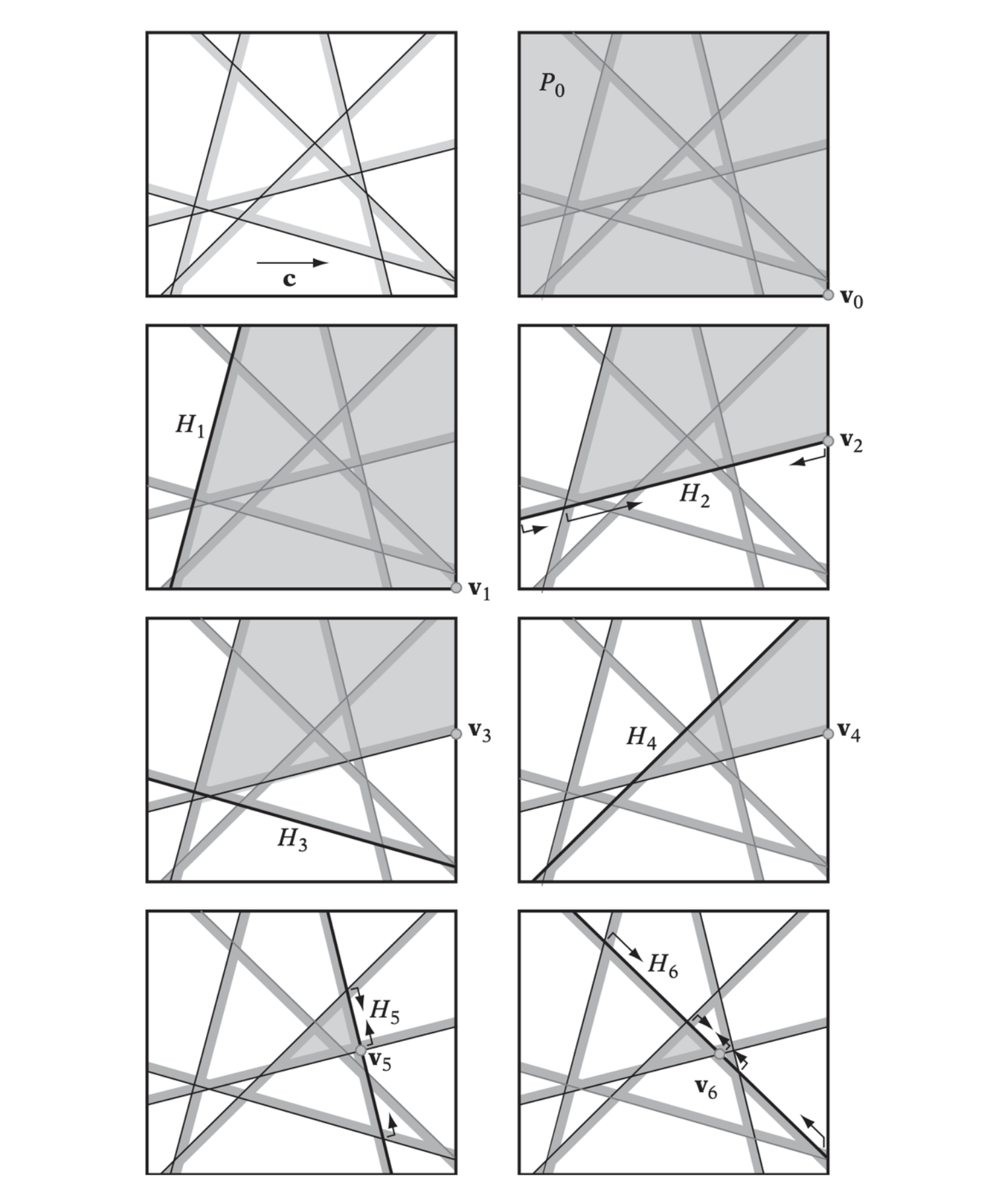
At top left, the six halfspaces from the two triangles given above. Remaining illustrations show Seidel’s algorithm applied to these six halfspaces. The feasible region is shown in light gray and the current halfspace is shown in thick black. Arrows indicate the 1D constraints in the recursive call.

The Gilbert-Johnson-Keerthi Algorithm

The GJK algorithm is one of the most effective methods for determining intersection between two polyhedra. GJK is an iterative and simplex-based descent algorithm that given two sets of vertices as inputs finds the Euclidean distance between the convex hulls of these sets.

The Algorithm

The algorithm is based on the fact that the separation distance between two polyhedra \(A\) and \(B\) is equivalent to the distance between their Minkowski difference \(C = A \ominus B\) and the origin. The key point of the GJK algorithm is that it does not explicitly compute the Minkowski difference \(C\). It only samples the Minkowski difference point set using a support mapping of \(C = A \ominus B\).

The distance between A and B is equivalent to the distance between their Minkowski difference and the origin.

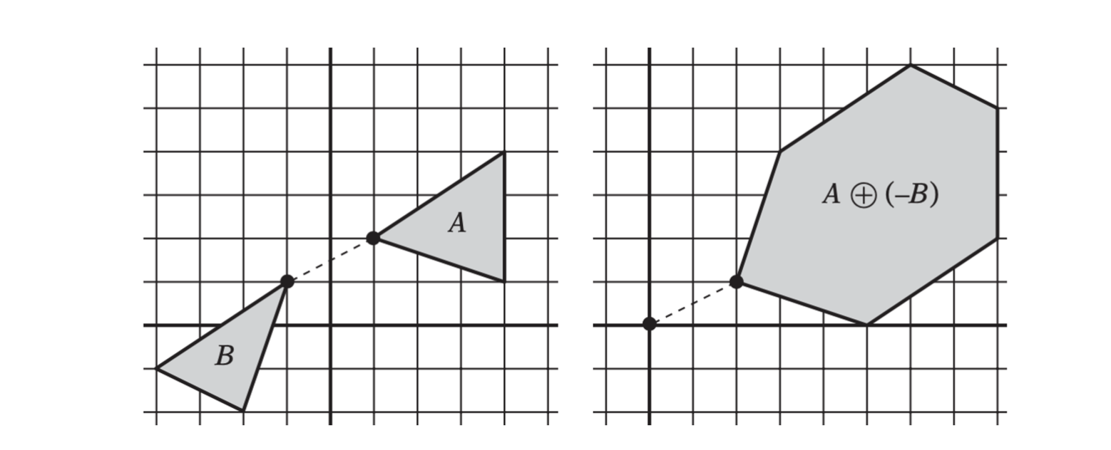
The distance between A and B is equivalent to the distance between their Minkowski difference and the origin.

A support mapping is a function \(s_A(\textbf{d})\) that maps a given direction \(\textbf{d}\) into a supporting point for the convex object \(A\) in that direction. Because the support mapping function is the maximum over a linear function, the support mapping for \(C, s_{A \ominus B}(\textbf{d})\), can be expressed in terms of the support mappings for \(A\) and \(B\) as \(s_{A \ominus B}(\textbf{d}) = s_A(\textbf{d}) - s_B(-\textbf{d})\). Thus, points from the Minkowski difference can be computed, on demand, from supporting points of the individual polyhedra \(A\) and \(B\).

The GJK Algorithm is stated as follows:

1. Initialize the simplex set \(Q\) to one or more points (up to \(d + 1\) points, where \(d\) is the dimension) from the Minkowski difference of \(A\) and \(B\).
2. Compute the point \(P\) of minimum norm in \(CH(Q)\).
3. If \(P\) is the origin itself, the origin is clearly contained in the Minkowski difference of \(A\) and \(B\). Stop and return \(A\) and \(B\) as intersecting.
4. Reduce \(Q\) to the smallest subset \(Q'\) of \(Q\) such that \(P \in CH(Q')\). That is, remove any points from \(Q\) not determining the subsimple of \(Q\) in which \(P\) lies.
5. Let \(V = s_{A \ominus B}(-P) = s_A(-P) - s_B(P)\) be a supporting point in direction \(-P\).
6. If \(V\) is no more extremal in direction \(-P\) than \(P\) itself, stop and return \(A\) and \(B\) as not intersecting. The length of the vector from the origin to \(P\) is the separation distance of \(A\) and \(B\).
7. Add \(V\) to \(Q\) and go to 2.

GJK finding the point on a polygon closest to the origin.

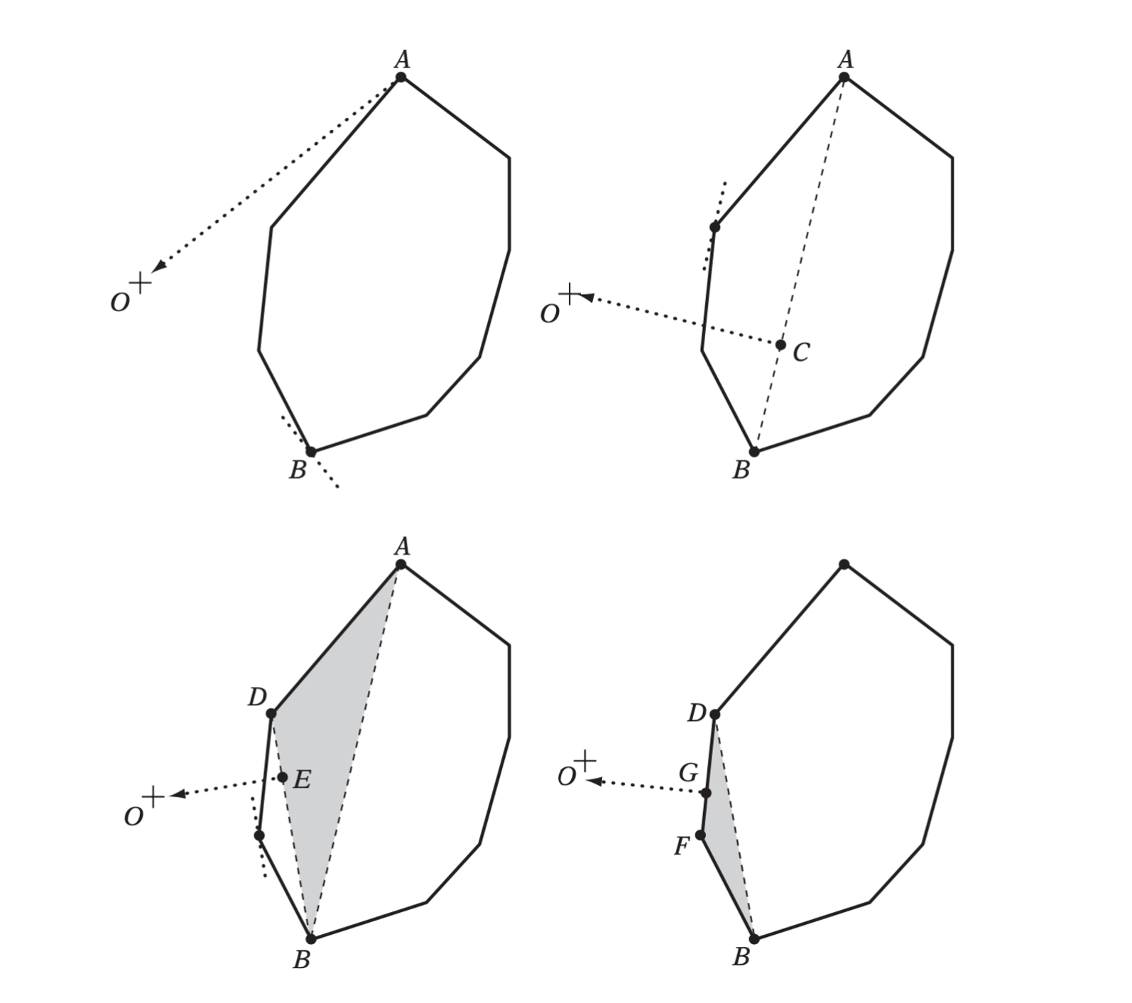
GJK finding the point on a polygon closest to the origin.

Finding the Point of Minimum Norm in a Simplex

Determining the point \(P\) of minimum norm in \(CH(Q)\) for a simplex set \(Q = \{Q_1, Q_2, \dots, Q_k\}, k \in [1, 4]\) can be done by the distance subalgorithm (Johnson’s algorithm). The distance algorithm reduces the problem to considering all subsets of \(Q\) separately. For \(k = 4\) there are 15 subsets.

• 4 vertices \((Q_1, Q_2, Q_3, Q_4)\)
• 6 edges \((Q_1Q_2, Q_1Q_3, Q_1Q_4, Q_2Q_3, Q_2Q_4, Q_3Q_4)\)
• 4 faces \((Q_1Q_2Q_3, Q_1Q_2Q_4, Q_1Q_3Q_4, Q_2Q_3Q_4)\)
• interior \((Q_1Q_2Q_3Q_4)\)

Once a feature has been located, the point of minimum norm on the feature is given by the orthogonal projection of the origin onto the feature.

Hill Climbing for Extreme Vertices

One of the most expensive steps of the GJK algorithm is finding an extreme vertex in a given direction. Trivially, extreme vertices can be located in \(O(n)\) time by searching over all \(n\) vertices. A better approach relis on having a data structure listing all adjacent vertex neighbors for each vertex. Then an extreme vertex can be found through a simple hill-climbing algorithm, greedily visiting more and more extreme vertices until no vertex more extreme can be found.

(a) Hill climbing from V to the most extreme vertex E (in direction d) using adjacent vertices only. (b) Accelerated hill climbing using additional (artificial adjacency) information.

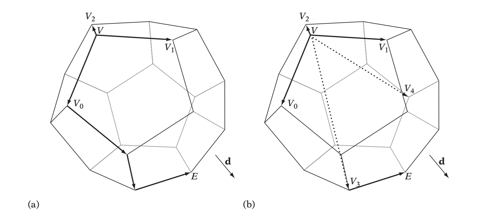
For larger polyhedra, the hill climbing can be sped up by adding one or more artificial neighbors to the adjacency list for a vertex. By linking to vertices at a greater distance away from the current vertex, the hill-climbing algorithm is likely to make faster progress toward the most extreme vertex when moving through these artificial vertices.

GJK for Moving Objects

Consider two polyhedra \(P\) and \(Q\), with movements given by the vectors \(\textbf{t}_1\) and \(\textbf{t}_2\), respectively. To simplify the collision test, the problem is recast so that \(Q\) is stationary. The relative movement of \(P\) (with respect to \(Q\)) is now given by \(\textbf{t} = \textbf{t}_1 - \textbf{t}_2\). Let \(V_i\) be the vertices of \(P\) in its initial position. \(V_i + \textbf{t}\) describes the location of the vertices of \(P\) at the end of its translational motion.

Determining if \(P\) collides with \(Q\) during its translational motion is therefore as simple as passing GJK the vertices of \(P\) at both the start and end of \(P\)’s motion.

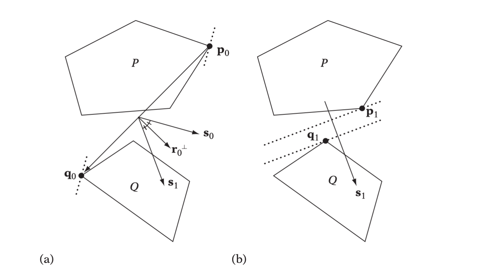
The Chung-Wang Separating-vector Algorithm

The CW algorithm operates on the vertices of the polyhedra. At each iteration \(i\), the main algorithm computes the two vertices \(\textbf{p}_i\) and \(\textbf{q}_i\) (\(\textbf{p}_i \in P, \textbf{q}_i \in Q\)) most extreme with resepect to the current candidate separating-vector \(\textbf{s}_i\). If this pair of vertices indicates object separation along \(\textbf{s}_i\), the algorithm exits with no intersection. Otherwise, the algorithm computes a new candidate separating vector by reflecting \(\textbf{s}_i\) about the perpendicular to the line through to \(\textbf{p}_i\) and \(\textbf{q}_i\). The algorithm is described as below:

1. Start with some candidate separating vector \(\textbf{s}_0\) and let \(i = 0\).
2. Find extreme vertices \(\textbf{p}_i\) of \(P\) and \(\textbf{q}_i\) of \(Q\) such that \(\textbf{p}_i \cdot \textbf{s}_i\) and \(\textbf{q}_i \cdot -\textbf{s}_i\) are maximized.
3. If \(\textbf{p}_i \cdot \textbf{s}_i < \textbf{q}_i \cdot -\textbf{s}_i\), then \(\textbf{s}_i\) is a separating axis. Exit reporting no intersection.
4. Otherwise, compute a new separating vector as \(\textbf{s}_{i+1} = \textbf{s}_i - 2(\textbf{r}_i \cdot \textbf{s}_i) \textbf{r}_i\), where \(\textbf{r}_i = (\textbf{q}_i - \textbf{p}_i)/ \| \textbf{q}_i - \textbf{p}_i\|\).
5. Let \(i = i + 1\) and go to 2.

(a) The first iteration of the CW algorithm for polygons P and Q. (b) A separating vector is found in the second iteration.