Spatial Partitioning

Spatial partitioning techniques provide broad-phase processing by dividing space into regions and testing if objects overlap the same region of space.

Uniform Grids

A very effective space subdivision scheme is to overlay space with a regular grid. The grid divides space into a number of regions, or grid cells, or equal size. Each object is then associated with the cells it overlaps.

Issues related to cell size. (a) A grid that is too fine. (b) A grid that is too coarse (with respect to object size). (c) A grid that is too coarse (with respect to object complexity). (d) A grid that is both too fine and too coarse.

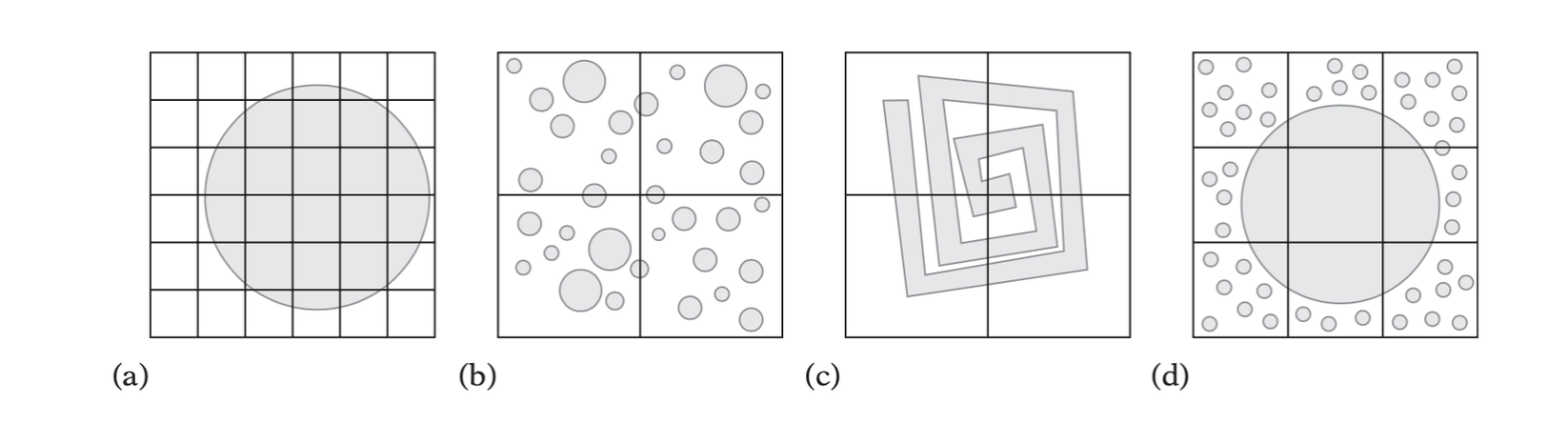
Cell Size Issues

• The grid is too fine. If the cells are too small, a large number of cells must be updated with associativity information for the object, which will take both extra time and space.
• The grid is too coarse (with respect to object size). If the objects are small and the grid cells are large, there will be many objects in each cell.
• The grid is too coarse (with respect to object complexity). In this case, the grid cell matches the objects well in size. However, the object is much too complex, affecting the pairwise object comparison.
• The grid is both too fine and too coarse. If the objects are of greatly varying sizes, the cells can be too large for the smaller objects while too small for th largest objects.

In ray tracing a popular method for determining the grid dimension has been the \(n^{1/3}\) rule: given \(n\) objects, divide space into a \(k \times k \times k\) grid, with \(k = n^{1/3}\). The ratio of cells to objects is referred to as the grid density.

Grids as Arrays of Linked Lists

The natural way of storing objects in a grid is to allocate an array of corresponding dimension, mapping grid cells to array elements one-to-one. To handle the case of multiple objects ending up in a given cell, each array element would point to a linked list of objects, or be NULL if empty.

💡 A drawback with using a dense array of this type is that for large grids just storing the list headers in each grid cell becomes projibitive in terms of memory requirements.

Hashed Storage and Infinite Grids

The most effective alternative to using a dense array to store the grid is to map each cell into a hash table of a fixed set of \(n\) buckets. In this scheme, the buckets contain the linked lists of objects.

A (potentially infinite) 2D grid is mapped via a hash function into a small number of hash buckets.

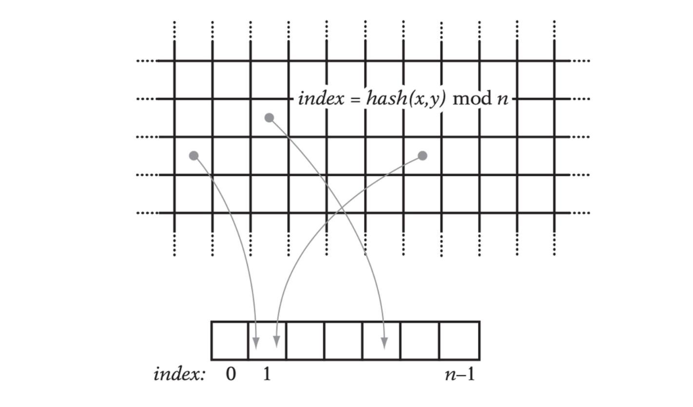
A (potentially infinite) 2D grid is mapped via a hash function into a small number of hash buckets.

// Cell position
struct Cell {
    Cell(int32 px, int32 py, int32 pz) { x = px; y = py; z = pz; }
    int32 x, y, z;
};

#define NUM_BUCKETS 1024

// Computes hash bucket index in range [0, NUM_BUCKETS-1]
int32 ComputeHashBucketIndex(Cell cellPos) {
    const int32 h1 = 0x8da6b343; // Large multiplicative constants
    const int32 h2 = 0xd8163841; // here arbitrarily chosen primes
    const int32 h3 = 0xcb1ab31f;
    int32 n = h1 * cellPos.x + h2 * cellPos.y + h3 * cellPos.z;
    n = n % NUM_BUCKETS;
    if (n < 0) n += NUM_BUCKETS;
    return n;
}

Although the world may consist of an infinite amount of cells, only a finite number of them are overlapped by objects at a given time. Thus, the storage required for a hashed grid is related to the number of objects and is independent of the grid size.

Storing Static Data

When the grid is static, the need for a linked list can be removed and all cell data can be stored in a single contiguous array.

(a) A grid storing static data as lists.(b)The same grid with the static data stored into an array.

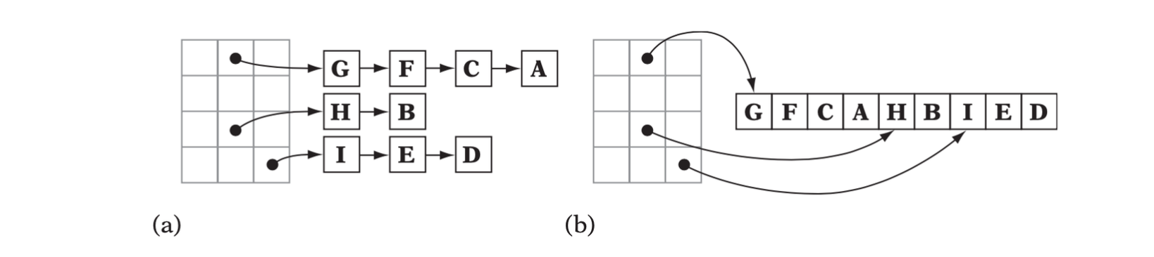
1. A grid storing static data as lists.(b)The same grid with the static data stored into an array.

Implicit Grids

As the Cartesian product of two or more arrays, the grid is now presented by two arrays (three in 3D), wherein one array corresponds to the grid rows and the other to the grid columns. An object is inserted into the grid by adding it to the lists of the grid cells it overlaps, for both the row and column array.

A 4 × 5 grid implicitly defined as the intersection of 9 (4 + 5) linked lists. Five objects have been inserted into the lists and their implied positions in the grid are indicated.

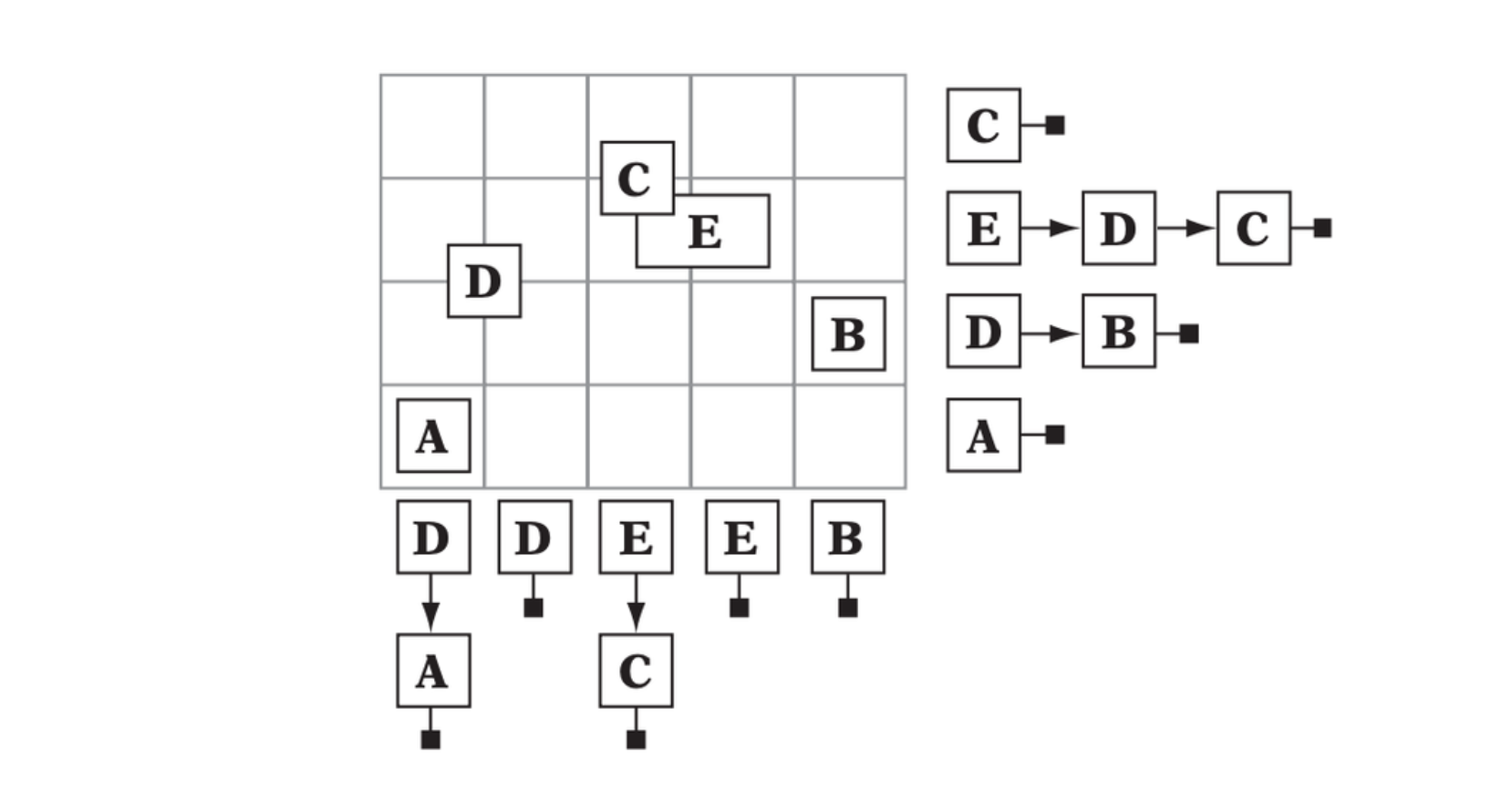
A 4 × 5 grid implicitly defined as the intersection of 9 (4 + 5) linked lists. Five objects have been inserted into the lists and their implied positions in the grid are indicated.

Uniform Grid Object-Object Test

Grid cell sizes are usually constrained to be larger than the largest object. This way, an object is guaranteed to overlap at most the immediately neighboring cells.

One Test at a Time

Consider the case in which objects are associated with a single cell only. When a given object is associated with its cell, in addition to testing agiasnt the objects associated with that cell additional neighboring cells must also be tested. Which cells have to be tested depends on how objects can overlap into other cells and what feature has been used to associate an object with its cell. The choice of feature generally stands between:

• the object bounding sphere center.
• the minimum (top leftmost) corner of the AABB.

If objects have been placed with respect to their centers, any object in the neighboring cells could overlap a cell boundary of this cell and be in collision with the current object.

// Objects placed in single cell based on their bounding sphere center.
// Checking object’s cell and all 8 neighboring grid cells:
check object’s cell
check northwest neighbor cell
check north neighbor cell
check northeast neighbor cell
check west neighbor cell
check east neighbor cell
check southwest neighbor cell
check south neighbor cell
check southeast neighbor cell

If instead the minimum corner of the AABB has been used, most neighboring cells have to be tested only if the current object actually overlaps into them.

// Objects placed in single cell based on AABB minimum corner vertex.
// Checking object’s "minimum corner" cell and up to all 8 neighboring grid cells: check object’s "minimum corner" cell
check north neighbor cell
check northwest neighbor cell
check west neighbor cell
if (object overlaps east cell border) {
    check northeast neighbor cell
    check east neighbor cell
}
if (object overlaps south cell border) {
    check southwest neighbor cell
    check south neighbor cell
    if (object overlaps east cell border)
        check southeast neighbor cell
}

If objects have been placed in all cells they overlap the single object test would have to check only those exact cells the AABB overlaps, as all colliding objects are guaranteed to be in those cells.

// Objects placed in all cells overlapped by their AABB.
// Checking object’s "minimum corner" cell and up to 3 neighboring grid cells:
check object’s "minimum corner" cell
if (object overlaps east cell border)
    check east neighbor cell
if (object overlaps south cell border) {
    check south neighbor cell
    if (object overlaps east cell border)
        check southeast neighbor cell
}

Objects A and B are assigned to a cell based on the location of their topleft-hand corners. In this case, overlap may occur in a third cell. Thus, to detect intersection between objects cells must be tested against their NE or SW neighbor cells.

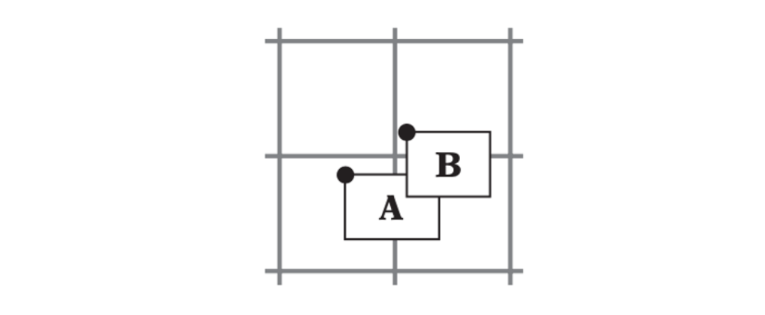
Objects A and B are assigned to a cell based on the location of their topleft-hand corners. In this case, overlap may occur in a third cell. Thus, to detect intersection between objects cells must be tested against their NE or SW neighbor cells.

All Tests at a Time

If instead of testing a single object at a time all objects are tested at the same time, the single-cell placement case can be optimized utilizing the fact that object pair checking is commutative.

💡 All neighbors now do not have to be checked. It is sufficient to check half the neighbors and let the remaining half of directionally opposing tests be covered by the communicativity relation.

If objects have been placed with respect to their centers

// Objects placed in single cell based on their bounding sphere center.
// All objects are checked for collisions at the same time, so collisions
// in the opposite direction will be handled when checking the objects // existing in those cells.
**check object’s cell
check east neighbor cell
check southwest neighbor cell
check south neighbor cell
check southeast neighbor cell**

The case in which objects are placed in a single cell based on the minimum corner point can be similarly simplified.

// Objects placed in single cell based on AABB minimum corner vertex.
// All objects are checked for collisions at the same time, so collisions // in the opposite direction will be handled when checking the objects
// existing in those cells.
check object’s "minimum corner" cell
check southwest neighbor cell
if (object overlaps east cell border)
    check east neighbor cell
if (object overlaps south cell border) {
    check south neighbor cell
    if (object overlaps east cell border)
        check southeast neighbor cell
}

Hierarchical Grids

The most significant problem with uniform grids is their inability to deal with objects of greatly varying sizes in a graceful way. The size problem can effectively be addressed by the use of hierarchical grids (or hgrids), a grid structure particularly well suited to holding dynamically moving objects.

Given a hierarchy containing \(n\) levels of grids and letting \(r_k\) represent the size of the grid cels at level \(k\) in the hierarchy, the grids are arranged in increasing cell size order, with \(r_1 < r_2 < \cdots < r_n\).

To minimize the number of neighboring cells that have to be tested for collisions objects are inserted into the hgrid at the level where the cells are large enough to contain the bounding volume of the object. Given an object \(P\), this level \(L\) is denoted \(L = \text{Level}(P)\). This way, the object is guaranteed to overlap at most four cells (or eight, for a 3D grid).

A small 1D hierarchical grid. Six objects, A through F, have each been inserted in the cell containing the object center point, on the appropriate grid level. The shaded cells are those that must be tested when performing a collision check for object C.

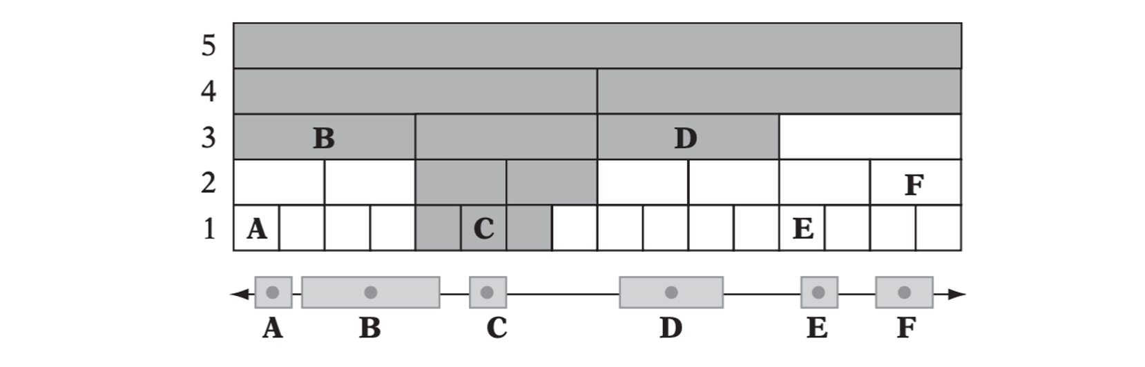
A small 1D hierarchical grid. Six objects, A through F, have each been inserted in the cell containing the object center point, on the appropriate grid level. The shaded cells are those that must be tested when performing a collision check for object C.

Let the cells at level 1 just encompass the smallest objects. Then successively double the cell size so that cells of level \(k + 1\) are twice as wide as cells of level \(k\). Repeat the doubling process until the highest-level cells are large enough to encompass the largest objects.

Basic Hgrid Implementation

The minimal structure of hgrid is as below:

struct HGrid {
    uint32 occupiedLevelsMask; // Initially zero (Implies max 32 hgrid levels) int objectsAtLevel[HGRID_MAX_LEVELS]; // Initially all zero
    Object *objectBucket[NUM_BUCKETS]; // Initially all NULL
    int timeStamp[NUM_BUCKETS]; // Initially all zero
    int tick;
};

It is assumed that objects are inserted into the hgrid based on their bounding spheres. Let the object representation contain the following variables.

struct Object {
    Object *pNextObject; // Embedded link to next hgrid object
    Point pos; // x, y (and z) position for sphere (or top left AABB corner))
    float radius; // radius for bounding sphere (or width of AABB)
    int bucket; // Index of hash bucket object is in
    int level; // Grid level for the object
    ... // Object data
}

Adding an Object

Adding an object into the hgrid can be done as follows.

void AddObjectToHGrid(HGrid *grid, Object *obj) {
    // Find lowest level where object fully fits inside cell, taking RATIO into account
    int level;
    float size = MIN_CELL_SIZE, diameter = 2.0f * obj->radius;
    for (level = 0; size * SPHERE_TO_CELL_RATIO < diameter; level++)
        size *= CELL_TO_CELL_RATIO;
    
    // Assert if object is larger than largest grid cell
    assert(level < HGRID_MAX_LEVELS);

    // Add object to grid square, and remember cell and level numbers,
    // treating level as a third dimension coordinate
    Cell cellPos((int)(obj->pos.x / size), (int)(obj->pos.y / size), level);
    int bucket = ComputeHashBucketIndex(cellPos);
    obj->bucket= bucket;
    obj->level = level;
    obj->pNextObject = grid->objectBucket[bucket];
    grid->objectBucket[bucket] = obj;
    
    // Mark this level as having one more object. Also indicate level is in use
    grid->objectsAtLevel[level]++;
    grid->occupiedLevelsMask |= (1 << level);
}

Removing an Object

Removing an object from the hgrid can be done in a corresponding manner.

void RemoveObjectFromHGrid(HGrid *grid, Object *obj) {
    // One less object on this grid level.
    // Mark level as unused if no objects left.
    if (--grid->objectsAtLevel[obj->level] == 0)
        grid->occupiedLevelsMask &= ∼(1 << obj->level);

    // Now scan through list and unlink object ’obj’
    int bucket= obj->bucket;
    Object *p = grid->objectBucket[bucket];
    // Special-case updating list header when object is first in list
    if (p == obj) {
        grid->objectBucket[bucket] = obj->pNextObject;
        return;
    }
    // Traverse rest of list, unlinking ’obj’ when found
    while (p) {
        // Keep q as trailing pointer to previous element
        Object *q = p;
        p = p->pNextObject;
        if (p == obj) {
            q->pNextObject = p->pNextObject;
            return;
        }
    }
    assert(0); // No such object in hgrid 
}

Checking an Object for Collision

Checking an object for collision against objects in the hgrid can be done as follows. It is assume that nothing is known about the number of objects tested at a time, and thus all grid levels are traversed.

// Test collisions between object and all objects in hgrid
void CheckObjAgainstGrid(
    HGrid *grid,
    Object *obj,
    void (*pCallbackFunc)(Object *pA, Object *pB)
) {
    float size = MIN_CELL_SIZE;
    int startLevel = 0;
    uint32 occupiedLevelsMask = grid->occupiedLevelsMask;
    Point pos = obj->pos;
    // If all objects are tested at the same time, the appropriate starting
    // grid level can be computed as:
    // float diameter = 2.0f * obj->radius;
    // for ( ; size * SPHERE_TO_CELL_RATIO < diameter; startLevel++)
    //     size *= CELL_TO_CELL_RATIO;
    //     occupiedLevelsMask >>= 1;
    // }

    // For each new query, increase time stamp counter
    grid->tick++;

    for (
        int level = startLevel;
        level < HGRID_MAX_LEVELS;
        size *= CELL_TO_CELL_RATIO, occupiedLevelsMask >>= 1, level++
    ) {
        // If no objects in rest of grid, stop now
        if (occupiedLevelsMask == 0) break;
        // If no objects at this level, go on to the next level
        if ((occupiedLevelsMask & 1) == 0) continue;

        // Compute ranges [x1..x2, y1..y2] of cells overlapped on this level. To
        // make sure objects in neighboring cells are tested, by increasing range by
        // the maximum object overlap: size * SPHERE_TO_CELL_RATIO
        float delta = obj->radius + size * SPHERE_TO_CELL_RATIO + EPSILON;
        float ooSize = 1.0f / size;
        int x1 = (int)floorf((pos.x - delta) * ooSize);
        int y1 = (int)floorf((pos.y - delta) * ooSize);
        int x2 = (int)ceilf((pos.x + delta) * ooSize);
        int y2 = (int)ceilf((pos.y + delta) * ooSize);

        // Check all the grid cells overlapped on current level
        for (int x = x1; x <= x2; x++) {
            for (int y = y1; y <= y2; y++) {
                // Treat level as a third dimension coordinate
                Cell cellPos(x, y, level);
                int bucket = ComputeHashBucketIndex(cellPos);

                // Has this hash bucket already been checked for this object?
                if (grid->timeStamp[bucket] == grid->tick) continue;
                grid->timeStamp[bucket] = grid->tick;

                // Loop through all objects in the bucket to find nearby objects
                Object *p = grid->objectBucket[bucket];
                while (p) {
                    if (p != obj) {
                        float dist2 = Sqr(pos.x - p->pos.x) + Sqr(pos.y - p->pos.y);
                        if (dist2 <= Sqr(obj->radius + p->radius + EPSILON))
                            pCallbackFunc(obj, p); // Close, call callback function 
                    }
                    p = p->pNextObject;
            }
        } // end for level
}

Trees

Trees form good representations for spatial partitioning.

Octrees (and Quadtrees)

The archetypal tree-based spatial partitioning method is the octree. It is an axis-aligned hierarchical partitioning of a volume of 3D world space.

• Each parent node has eight children.
• Each node has a finite volume associated with it.
• The root node volume is taken to be the smallest AABB fully enclosing the world. The volume is then subdivided into eight smaller equal-size subcubes.

The octree node data structure is as below.

// Octree node data structure
struct Node {
    Point center; // Center point of octree node (not strictly needed)
    float halfWidth; // Half the width of the node volume (not strictly needed)
    Node *pChild[8]; // Pointers to the eight children nodes
    Object *pObjList; // Linked list of objects contained at this node
};

Octree Object Assignment

Octrees may be built to contain either static or dynamic data.

• The data may be the primitives forming the world environment.
• The data may by the moving entities in the world.

A quad tree node with the first level of subdivision shown in black dotted lines, and the following level of subdivision in gray dashed lines. Dark gray objects overlap the first- level dividing planes and become stuck at the current level. Medium gray objects propagate one level down before becoming stuck. Here, only the white objects descend two levels.

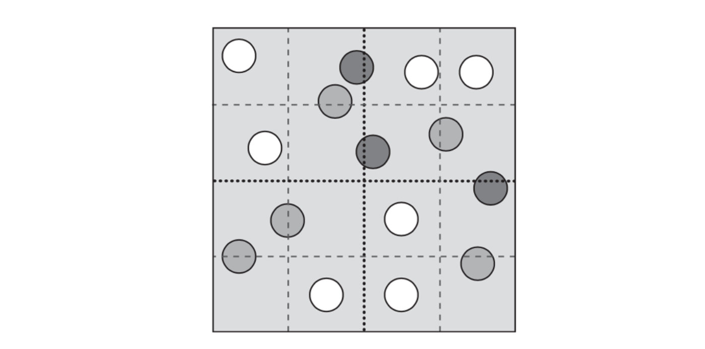
A quad tree node with the first level of subdivision shown in black dotted lines, and the following level of subdivision in gray dashed lines. Dark gray objects overlap the first- level dividing planes and become stuck at the current level. Medium gray objects propagate one level down before becoming stuck. Here, only the white objects descend two levels.

The process of building an octree is as below.

// Preallocates an octree down to a specific depth
Node *BuildOctree(Point center, float halfWidth, int stopDepth) {
    if (stopDepth < 0) return NULL;

    else {
        // Construct and fill in ’root’ of this subtree
        Node *pNode = new Node;
        pNode->center = center;
        pNode->halfWidth = halfWidth;
        pNode->pObjList = NULL;
        // Recursively construct the eight children of the subtree
        Point offset;
        float step = halfWidth * 0.5f;
        for (int i = 0; i < 8; i++) {
            offset.x = ((i & 1) ? step : -step);
            offset.y = ((i & 2) ? step : -step);
            offset.z = ((i & 4) ? step : -step);
            pNode->pChild[i] = BuildOctree(center + offset, step, stopDepth - 1);
        }
        return pNode;
    }
}

The structure of the object is as follows.

struct Object {
    Point center; // Center point for object
    float radius; // Radius of object bounding sphere
    ...
    Object *pNextObject; // Pointer to next object when linked into list
}

Octree Object Insertion

The code for inserting an object is as follows.

void InsertObject(Node *pTree, Object *pObject) {
    int index = 0, straddle = 0;
    // Compute the octant number [0..7] the object sphere center is in
    // If straddling any of the dividing x, y, or z planes, exit directly
    for (int i = 0; i < 3; i++) {
        float delta = pObject->center[i] - pTree->center[i];
        if (Abs(delta) < pTree->halfWidth + pObject->radius) {
            straddle = 1;
            break;
        }
        if (delta > 0.0f) index |= (1 << i); // ZYX
    }
    if (!straddle && pTree->pChild[index]) {
        // Fully contained in existing child node; insert in that subtree
        InsertObject(pTree->pChild[index], pObject);
    } else {
        // Straddling, or no child node to descend into, so
        // link object into linked list at this node
        pObject->pNextObject = pTree->pObjList;
        pTree->pObjList = pObject;
    }
}

Octree Object Collision Test

// Tests all objects that could possibly overlap due to cell ancestry and coexistence
// in the same cell. Assumes objects exist in a single cell only, and fully inside it
void TestAllCollisions(Node *pTree) {
    // Keep track of all ancestor object lists in a stack
    const int MAX_DEPTH = 40;
    static Node *ancestorStack[MAX_DEPTH];
    static int depth = 0; // ’Depth == 0’ is invariant over calls

    // Check collision between all objects on this level and all
    // ancestor objects. The current level is included as its own
    // ancestor so all necessary pairwise tests are done ancestorStack[depth++] = pTree;
    for (int n = 0; n < depth; n++) {
        Object *pA, *pB;
        for (pA = ancestorStack[n]->pObjList; pA; pA = pA->pNextObject) {
            for (pB = pTree->pObjList; pB; pB = pB->pNextObject) {
                // Avoid testing both A->B and B->A
                if (pA == pB) break;
                // Now perform the collision test between pA and pB in some manner
                TestCollision(pA, pB);
            }
    }
    }
    
    // Recursively visit all existing children
    for (int i = 0; i < 8; i++)
        if (pTree->pChild[i])
            TestAllCollisions(pTree->pChild[i]);
    
    // Remove current node from ancestor stack before returning
    depth--;
}

Loose Octrees

An effective way of dealing with straddling objects is to expand the node volumes by some amount to make them partially overlapping. The resulting relaxed octrees have been dubbed loose octrees.

(a) The cross section of a regular octree, shown as a quad tree.(b) Expanding the nodes of the octree, here by half the node width in all directions, turns the tree into a loose octree. (The loose nodes are offset and shown in different shades of gray to better show their boundaries. The original octree nodes are shown as dashed lines.)

k-d Trees

A generalization of octrees and quadtrees can be found in the k-dimensional tree, or k-d tree. Here, \(k\) represents the number of dimensions subdivided, which does not have to match the dimensionality of the space used.

Instead of simultaneously dividing space in two or three dimensions, the k-d tree divides space along one dimension at a time. One level of an octree can be seen as a three-level k-d tree split along x, then y, then z.

A 2D k-d tree.(a)The spatial decomposition. (b) The k-d tree layout.

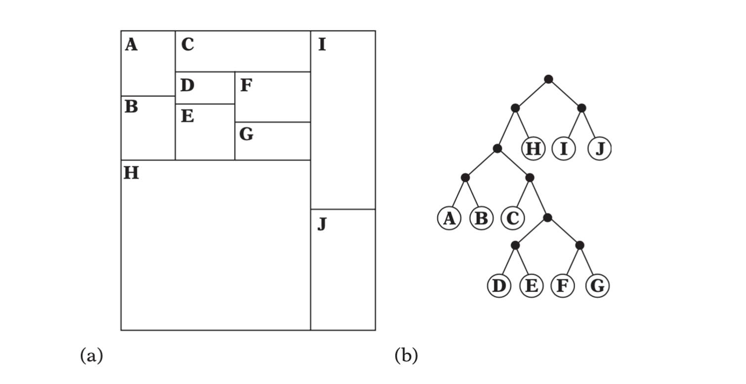
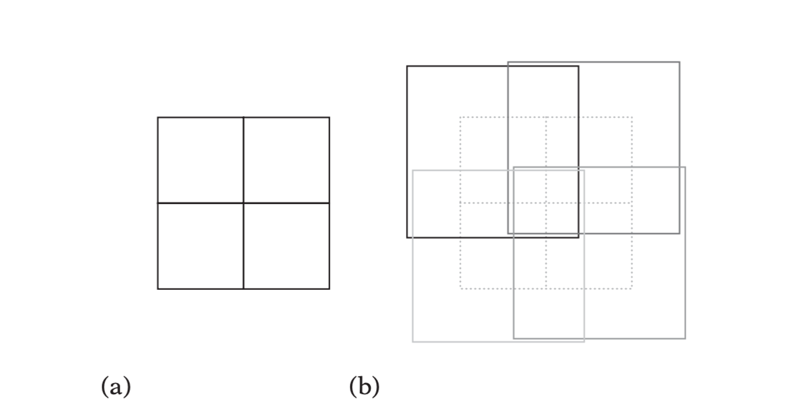
A 2D k-d tree.(a)The spatial decomposition. (b) The k-d tree layout.

Usage of k-d tree

• whenever quadtrees or octrees are used.
• point location (given a point, locate the region it is in).
• nearest neighbor (find the point in a set of points the query point is closed to).
• range search (locate all points within a given region).

struct KDNode {
    KDNode *child[2]; // 0 = near, 1 = far
    int splitType; // Which axis split is along (0, 1, 2, ...)
    float splitValue; // Position of split along axis
    ...
};

// Visit k-d tree nodes overlapped by sphere. Call with volNearPt = s->c
void VisitOverlappedNodes(KDNode *pNode, Sphere *s, Point &volNearPt) {
    if (pNode == NULL) return;
    
    // Visiting current node, perform work here
    ...
    // Figure out which child to recurse into first (0 = near, 1 = far)
    int first = s->c[pNode->splitType] > pNode->splitValue;
    
    // Always recurse into the subtree the sphere center is in
    VisitOverlappedNodes(pNode->child[first], s, volNearPt);
    
    // Update (by clamping) nearest point on volume when traversing far side.
    // Keep old value on the local stack so it can be restored later
    float oldValue = volNearPt[pNode->splitType];
    volNearPt[pNode->splitType] = pNode->splitValue;
    
    // If sphere overlaps the volume of the far node, recurse that subtree too
    if (SqDistPointPoint(volNearPt, s->c) < s->r * s->r)
        VisitOverlappedNodes(pNode->child[first ∧ 1], s, volNearPt);
    
    // Restore component of nearest pt on volume when returning
    volNearPt[pNode->splitType] = oldValue;
}

Hybrid Schemes

Hybrid schemes are the combination of using different techniques and strategies to divide the scene into multiple layers. For instance, after having initially assigned objects or geometry primitives to a uniform grid, the data in each nonempty grid cell could be further organized in a tree structure.

(a) A grid of trees, each grid cell containing a separate tree. (b) A grid indexing into a single tree hierarchy, each grid cell pointing into the tree at which point traversal should start.

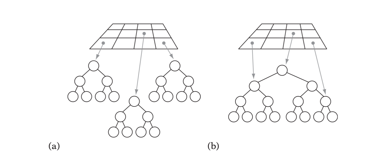
1. A grid of trees, each gridcellcontainingaseparatetree.(b)Agridindexing into a single tree hierarchy, each grid cell pointing into the tree at which point traversal should start.

Ray and Directed Line Segment Traversals

Particularly common in many applications, games in particular, are line pick tests. These are queries involving rays or directed line segments.

k-d Tree Intersection Test

The basic idea behind intersecting a ray or directed line segment with a k-d tree is straightforward. The segment \(S(t) = A + t\textbf{d}\) is intersected against the node’s splitting plane, and the \(t\) value of intersection is computed. It \(t\) is within the interval of the segment, \(0 \leq t \leq t_\text{max}\), the segment straddles the plane and both children of the tree are recursively descended.

// Visit all k-d tree nodes intersected by segment S = a + t * d, 0 <= t < tmax
void VisitNodes(KDNode *pNode, Point a, Vector d, float tmax) {
    if (pNode == NULL) return;

    // Visiting current node, perform actual work here
    ...

    // Figure out which child to recurse into first (0 = near, 1 = far)
    int dim = pNode->splitType;
    int first = a[dim] > pNode->splitValue;

    if (d[dim] == 0.0f) {
        // Segment parallel to splitting plane, visit near side only
        VisitNodes(pNode->child[first], a, d, tmax);
    } else {
        // Find t value for intersection between segment and split plane
        float t = (pNode->splitValue - a[dim]) / d[dim];
        // Test if line segment straddles splitting plane
        if (0.0f <= t && t < tmax) {
            // Yes, traverse near side first, then far side
            VisitNodes(pNode->child[first], a, d, t);
            VisitNodes(pNode->child[first ∧ 1], a + t * d, d, tmax - t);
        } else {
            // No, so just traverse near side
            VisitNodes(pNode->child[first], a, d, tmax);
        }
    }
}

Uniform Grid Intersection Test

The traversal method used must enforce 6-connectivity of the cells visited along the line. Cells in 3D are said to be 6-connected if they share faces only with other cells. If cells are also allowed to share edges, they are considered 18 connected. A cell is 26-connected if it can share a face, edge, or vertex with another cell.

Cell connectivity for a 2D line. (a) An 8-connected line. (b) A 4-connected line. In 3D, the corresponding lines would be 26-connected and 6-connected, respectively.

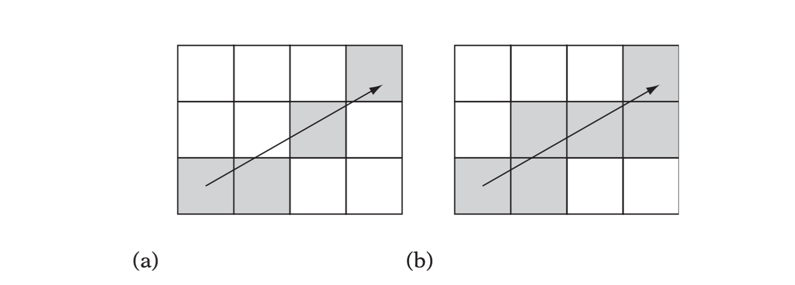
Cell connectivity for a 2D line. (a) An 8-connected line. (b) A 4-connectedline. In 3D, the corresponding lines would be 26-connected and 6-connected, respectively.

Sort and Sweep Methods

A drawback of inserting objects into the fixed spatial subdivisions that grids and octrees represent is having to deal with the added complications of objects straddling multiple partitions. An alternative approach is to instead maintain the objects in some sort of sorted spatial ordering. One way of spatially sorting the objects is the sort and sweep method.

Sorted Linked-list Implementation

To maintain the axis-sorted lists of projection interval extents, two types of structures are required: one that is the linked-list element corresponding to the minimum or maximum interval values and another one to link the two entries.

struct AABB {
    Elem min; // Element containing the three minimum interval values
    Elem max; // Element containing the three maximum interval values
    Object *pObj; // Pointer to the actual object contained in the AABB
};

struct Elem {
    Elem *pLeft[3]; // Pointers to the previous linked list element (one for each axis)
    Elem *pRight[3]; // Pointers to the next linked list element (one for each axis)
    float value[3]; // All min or all max coordinate values (one for each axis)
    int minmax:1; // All min values or all max values?
};

Cells and Portals

This method was developed for rendering architectural walkthrough systems. The cells-and-portals method exploits the occluded nature of these scenes to reduce the amount of geometry that has to be rendered. The method proceeds by dividing the world into regions (cells) and the boundaries that connect them (portals). Rooms in the scene would correspond to cells, and doorways and windows to portals.

A simple portalized world with five cells (numbered) and five portals (dashed). The shaded region indicates what can be seen from a given viewpoint. Thus, here only cells 2, 3, and 5 must be rendered.

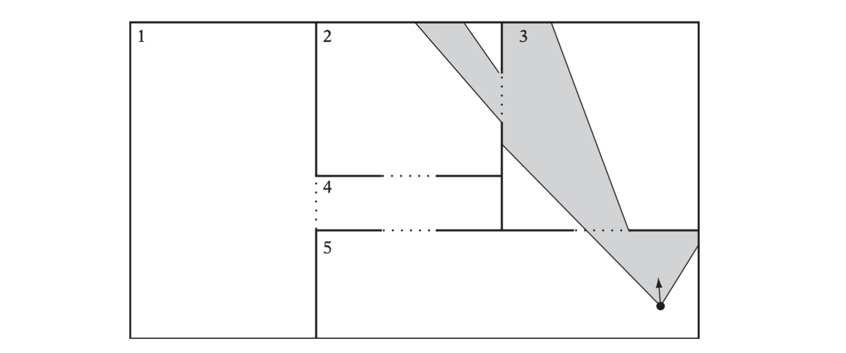
A simple portalized world with five cells (numbered) and five portals (dashed). The shaded region indicates what can be seen from a given viewpoint. Thus, here only cells 2, 3, and 5 must be rendered.

Rendering a scene partitioned into cells and portals starts with drawing the geometry for the cell containing the camera. After this cell has been rendered, the rendering function is called recursively for adjoining cells whose portals are visible to the camera. During recursion, new portals encountered are clipped against the current portal, narrowing the view into the scene. Recursion stops when either the clipped portal becomes empty, or when no unvisited neighboring cells are available.

The following pseudocode illustrates an implementation of this rendering procedure.

RenderCell(ClipRegion r, Cell *c) {
    // If the cell has not already been visited this frame...
    if (c->lastFrameVisited != currentFrameNumber) {
        // ...timestamp it to make sure it is not visited several
        // times due to multiple traversal paths through the cells c->lastFrameVisited = currentFrameNumber;
        // Recursively visit all connected cells with visible portals
        for (Portal *pl = c->pPortalList; pl != NULL; pl = pl->pNextPortal) {
            // Clip the portal region against the current clipping region
            ClipRegion visiblePart = ProjectAndIntersectRegion(r, pl->boundary);
            // If portal is not completely clipped its contents must be partially
            // visible, so recursively render other side through the reduced portal
            if (!EmptyRegion(visiblePart))
                RenderCell(visiblePart, pl->pAdjoiningCell);
        }

        // Now render all polygons (done last, for back-to-front rendering)
        for (Polygon *p = c.pPolygonList; p != NULL; p = p->pNextPolygon)
            RenderPolygon(p);
    }
}