Bounding Volume Hierarchies

By arranging the bounding volumes into a tree hierarchy called a bounding volume hierarchy (BVH), the time complexity can be reduced to logarithmic in the number of tests performed.

A bounding volume hierarchy of five simple objects. Here the bounding volumes used are AABBs.

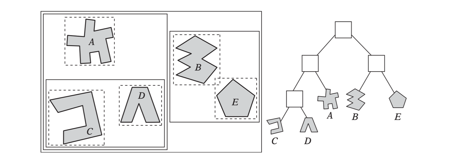
A bounding volume hierarchy of five simple objects. Here the bounding volumes used are AABBs.

With a hierarchy in place, during collision testing children do not have to be examined if their parent volume is not intersected.

Hierarchy Design Issues

Serval desired properties for bounding volume hierarchies have been suggested.

• The nodes contained in any given subtree should be near each other.
• Each node in the hierarchy should be of minimal volume.
• The sum of all bounding volumes should be minimal.
• Greater attention should be paid to nodes near the root of the hierarchy.
• The volume of overlap of sibling nodes should be minimal.
• The hierarchy should be balanced with respect to both its node structure and its content.

💡 For real-time applications, games especially, an important addition to the previous list is the requirement that the worse case time for queries not be much worse than the average case query time.

Cost Functions

The cost function is defined as below:

\[ T = N_VC_V + N_PC_P + N_UC_U + C_O \]

Here,

• \(T\) is the total cost of intersecting the two hierarchies
• \(N_V\) is the number of BV pairs tested for overlap
• \(C_V\) is the cost of testing a pair of BVs for overlap
• \(N_P\) is the number of primitive pairs tested
• \(C_P\) is the cost of testing a primitive pair
• \(N_U\) is the number of nodes that need to be updated
• \(C_U\) is the cost of updating each such node
• \(C_O\) is the cost of a one-time processing (such as a coordinate transformation between objects)

Tree Degree

In terms of size, a d-ary tree of \(n\) leaves has \((n - 1)/(d - 1)\) internal nodes for a total of \((nd - 1)/(d - 1)\) nodes in the tree.

Building Strategies for Hierrachy Construction

There are three primary categories of tree construction methods: top-down, bottom-up, and insertion methods.

A small tree of four objects built using (a) top-down, (b) bottom-up, and (c) insertion construction.

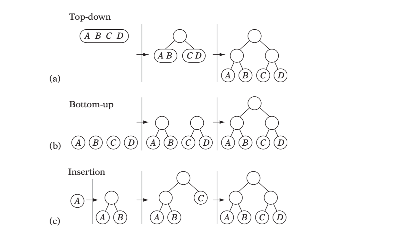
A small tree of four objects built using (a) top-down, (b) bottom-up, and (c) insertion construction.

Top-down Construction

It starts out by bounding the input set of primitives in a bounding volume. These primitives are then partitioned into two subsets. The procedure is now called recursively to form subhierarchies for the two subsets, which are then connected as children to the parent volume.

// Construct a top-down tree. Rearranges object[] array during construction
void TopDownBVTree(Node **tree, Object object[], int numObjects) {
    assert(numObjects > 0);
    const int MIN_OBJECTS_PER_LEAF = 1;
    Node *pNode = new Node;
    *tree = pNode;
    // Compute a bounding volume for object[0], ..., object[numObjects - 1]
    pNode->BV = ComputeBoundingVolume(&object[0], numObjects);
    if (numObjects <= MIN_OBJECTS_PER_LEAF) {
        pNode->type = LEAF;
        pNode->numObjects = numObjects;
        pNode->object = &object[0]; // Pointer to first object in leaf
    } else {
        pNode->type = NODE;
        // Based on some partitioning strategy, arrange objects into
        // two partitions: object[0..k-1], and object[k..numObjects-1]**
        int k = PartitionObjects(&object[0], numObjects);
        // Recursively construct left and right subtree from subarrays and
        // point the left and right fields of the current node at the subtrees
        TopDownBVTree(&(pNode->left), &object[0], k);
        TopDownBVTree(&(pNode->right), &object[k], numObjects - k);
    }
}

Partitioning Strategies

A simple partitioning method is the medium-cut-algorithm. Here, the set is divided in two equal size parts with respect to their projection along the selected axis, resulting in a balanced tree.

Other possible partition strategies are:

• Minimize the sum of the volumes of the child volumes.
• Minimize the maximum volume of the child volumes.
• Minimize the volume of the intersection of the child volumes.
• Maximize the separation of child volumes.
• Divide primitives equally between the child volumes.
• Combinations of the previous strategies.

Partitioning stops and a node is considered a leaf when some particular stop criterion is reached. Common stop criteria are:

• The node contains just a single primitive, or less than some k primitives.
• The volume of the bounding volume has fallenbelow a set cut-off limit.
• The depth of the node has reached a predefind cut-off depth.

Partitioning can also fail early, before a stop criterion triggers, for instance when:

• All primitives fall on one side of the split plane.
• One or both child volumes end up with as many (or nearly as many) primitives as the parent volume.
• Both child volumes are almost as large as the parent volume.

Choice of Partitioning Axis

Common choices of axes are:

• Local x, y, z coordinate axes.
• Axes from the intended aligned bounding volume.
• Axes of the parent bounding volume.
• Axis through the two most distant points.
• Axis along which variance is greatest.

💡 Even though a full optimization step is infeasible, once a partitioning axis has been selected a small number of hill-climbing steps can be performed to improve on the axis.

Choice of Split Point on the Partitioning Axis

• Median of the centroid coordinates (object median).
• Mean of the centroid coordinates (object mean).
• Median of the bounding volume projection extents (spatial median).
• Splitting at k evenly spaced points along the bounding volume projection extents. This brute force alternative simply tests some small number of evenly spaced points along the axis, picking the best one.
• Splitting between (random subset of ) the centroid coordinates.

(a) Splitting at the object median. (b) Splitting at the object mean. (c) Splitting at the spatial median.

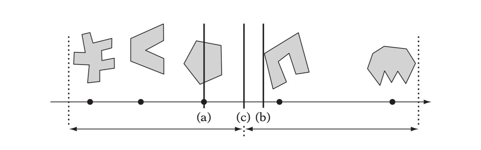
1. Splitting at the object median. (b) Splitting at the object mean. (c) Splitting at the spatial median.

Bottom-up Construction

In contrast to top-down methods, bottom-up methods are more complicated to implement and have a slower construction time but usually produce the best tress. To construct a tree hierarchy bottom up, the first step is to enclose each primitive within a bounding volume. These volumes form the leaf nodes of the tree. From the resulting set of volumes, two leaf nodes are selected based on some merging criterion (or called a clustering rule). These nodes are then bound within a bounding volume, which replaces the original nodes in the set. This pairing procedure repeats until the set consists of a single bounding volume representing the root node of the constructed tree.

Node *BottomUpBVTree(Object object[], int numObjects) {
    assert(numObjects != 0);
    int i, j;
    // Allocate temporary memory for holding node pointers to
    // the current set of active nodes (initially the leaves)
    NodePtr *pNodes = new NodePtr[numObjects];

    // Form the leaf nodes for the given input objects
    for (i = 0; i < numObjects; i++) {
        pNodes[i] = new Node;
        pNodes[i]->type = LEAF;
        pNodes[i]->object = &object[i];
    }
    // Merge pairs together until just the root object left
    while (numObjects > 1) {
        // Find indices of the two "nearest" nodes, based on some criterion
        FindNodesToMerge(&pNodes[0], numObjects, &i, &j);
        // Group nodes i and j together under a new internal node
        Node *pPair = new Node;
        pPair->type = NODE;
        pPair->left = pNodes[i];
        pPair->right = pNodes[j];
        // Compute a bounding volume for the two nodes
        pPair->BV = ComputeBoundingVolume(pNodes[i]->object, pNodes[j]->object);
        // Remove the two nodes from the active set and add in the new node.
        // Done by putting new node at index ’min’ and copying last entry 
        // to ’max’ int min = i, max = j;
        if (i > j) min = j, max = i;
        pNodes[min] = pPair;
        pNodes[max] = pNodes[numObjects - 1];
        numObjects--;
    }
    // Free temporary storage and return root of tree
    Node *pRoot = pNodes[0];
    delete pNodes;
    return pRoot;
}

An improved method using priority queue is shown as below.

Node *BottomUpBVTree(Object object[], int numObjects) {
    PriorityQueue<Pair> q;
    InsertionBVTree t;
    // Bound all objects in BV, forming leaf nodes. Insert leaf nodes into a
    // dynamically changable insertion-built BV tree
    InitializeInsertionBVTree(t, object, numObjects);

    // For all nodes, form pair of references to the node and the node it pairs
    // best with (resulting in the smallest bounding volume). Add all pairs to
    // the priority queue, sorted on increasing volume order
    InitializePriorityQueue(q, object, numObjects);

    while (SizeOf(q) > 1) {
        // Fetch the smallest volume pair from the queue
        Pair *p = Dequeue(q);

        // Discard pair if the node has already been paired
        if (HasAlreadyBeenPaired(p->node)) continue;

        // Recompute the best pairing node for this node to see if
        // the stored pair node is still valid
        Node *bestpairnode = ComputeBestPairingNodeUsingTree(t, p->node);
        if (p->pairnode == bestpairnode) {
            // The store pair node is OK, pair the two nodes together;
            // link the nodes together under a new node
            Node *n = new Node;
            n->left = p->node;
            n->right = p->pairnode;

            // Add new node to BV tree; delete old nodes as not possible to pair with
            Delete(t, p->node);
            Delete(t, p->pairnode);
            Insert(t, n);

            // Compute a pairing node for the new node; insert it into queue
            Node *newbestpairnode = ComputeBestPairingNodeUsingTree(t, n);
            p = Pair(n, newbestpairnode);
        } else {
            // Best pair node changed since the pair was inserted;
            // update the pair, reinsert into queue and try again
            p = Pair(p->node, bestpairnode);
        }
        Enqueue(q, p, VolumeOfBVForPairedNodes(p));
    }
    return Dequeue(q)->node;
}

Other Bottom-up Construction Strategies

Locating the point (or object) out of a set of points closest to a given query point is known as the nearest neighbor problem.

For forming larger clusters of objects, specific clustering algorithms can be used. One such approach is to treat the objects as vertices of a complete graph and compute a minimum spanning tree (MST) for the graph, with edge weights set to the distance between the two connected objects or some similar clustering measure. The MST can be computed using Prim’s algorithm or Kruskal’s algorithm.

Hierarchy Traversal

The two most fundamental tree-traversing methods are breadth-first search and depth-first search.

(a) Breadth-firstsearch, (b) depth-firstsearch, and (c) one possible best-firstsearch ordering.

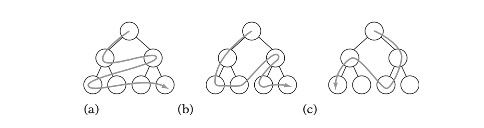
1. Breadth-firstsearch, (b) depth-firstsearch, and (c) one possible best-firstsearch ordering.

Pure breadth-first and depth-first traversals are considered uninformed or blind search methods. Uninformed search methods do not examine and make traversal decisions based on the data contained in the traversed structure. In contrast to the uninformed methods is the group of informed search methods. These attempt to utilize known information about the domain being searched through heuristic rules.

Generic Informed Depth-first Traversal

A generic informed depth-first traversal is as follows:

// Generic recursive BVH traversal code.
// Assumes that leaves too have BVs
void BVHCollision(CollisionResult *r, BVTree a, BVTree b) {
    if (!BVOverlap(a, b)) return;
    if (IsLeaf(a) && IsLeaf(b)) {
        // At leaf nodes. Perform collision tests on leaf node contents
        CollidePrimitives(r, a, b);
    } else {
        if (DescendA(a, b)) {
            BVHCollision(a->left, b);
            BVHCollision(a->right, b);
        } else {
            BVHCollision(a, b->left);
            BVHCollision(a, b->right);
        }
    }
}

In the code

• BVOverlap() determines the overlap between two bounding volumes.
• IsLeaf() return true if its argument is a leaf node and not an internal node.
• CollidePrimitives() collides all contained primitives against one another. Accumulating any reported collisions to the supplied CollisionResult structure.
• DescendA() implements the descent rule, and returns true if object hierarchy \(A\) should be descended or false for object hierarchy \(B\).

Some basic implementations of DescendA is shown as below.

// ‘Descend A’ descent rule
bool DescendA(BVTree a, BVTree b) {
    return !IsLeaf(a);
}

// ‘Descend B’ descent rule
bool DescendA(BVTree a, BVTree b) {
    return IsLeaf(b);
}

// ‘Descend larger’ descent rule
bool DescendA(BVTree a, BVTree b) {
    return IsLeaf(b) || (!IsLeaf(a) && (SizeOfBV(a) >= SizeOfBV(b)));
}

Simultaneous Depth-first Traversal

// Recursive, simultaneous traversal
void BVHCollision(CollisionResult *r, BVTree a, BVTree b) {
    if (!BVOverlap(a, b)) return;
    if (IsLeaf(a)) {
        if (IsLeaf(b)) {
            // At leaf nodes. Perform collision tests on leaf node contents
            CollidePrimitives(r, a, b);
            // Could have an exit rule here (eg. exit on first hit)
        } else {
            BVHCollision(a, b->left);
            BVHCollision(a, b->right);
        }
    } else {
        if (IsLeaf(b)) {
            BVHCollision(a->left, b);
            BVHCollision(a->right, b);
        } else {
            BVHCollision(a->left, b->left);
            BVHCollision(a->left, b->right);
            BVHCollision(a->right, b->left);
            BVHCollision(a->right, b->right);
        } 
    }
}

Merging Bounding Volumes

During bottom-up construction an alternative to the rather costly operation of fitting the bounding volume directly to the data is to merge the child volumes themselves into a new bounding volume.

Merging Two AABBs

// Computes the AABB a of AABBs a0 and a1
void AABBEnclosingAABBs(AABB &a, AABB a0, AABB a1) {
    for (int i = 0; i < 2; i++) {
        a.min[i] = Min(a0.min[i], a1.min[i]);
        a.max[i] = Max(a0.max[i], a1.max[i]);
    }
}

Merging Two Spheres

The calculation is best split into two cases:

• Either sphere is fully enclosed by the other.
• They are either partially overlapping or disjoint.

Let two sphere \(S_0\) and \(S_1\), the distance between two centers is \(d = \| C_1 - C_0 \|\). If \(|d_1 - d_0| \geq d\), then one sphere is fully inside the other.

Merging spheres S0 and S1.

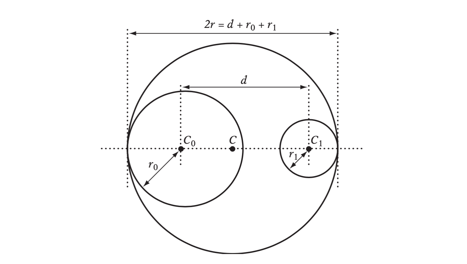
Merging spheres S0 and S1.

// Computes the bounding sphere s of spheres s0 and s1
void SphereEnclosingSpheres(Sphere &s, Sphere s0, Sphere s1) {
    // Compute the squared distance between the sphere centers
    Vector d = s1.c - s0.c;
    float dist2 = Dot(d, d);

    if (Sqr(s1.r - s0.r) >= dist2) {
        // The sphere with the larger radius encloses the other;
        // just set s to be the larger of the two spheres
        if (s1.r >= s0.r)
            s = s1;
        else
            s = s0;
    } else {
        // Spheres partially overlapping or disjoint
        float dist = Sqrt(dist2);
        s.r = (dist + s0.r + s1.r) * 0.5f;
        s.c = s0.c;
        if (dist > EPSILON)
            s.c += ((s.r - s0.r) / dist) * d;
    }
}

Efficient Tree Representation and Traversal

Array Representation

// First level
array[0] = *(root);

// Second level
array[1] = *(root->left);
array[2] = *(root->right);

// Third level
array[3] = *(root->left->left); ...

A binary tree (top) stored using a pointerless array representation (bottom). Children of node at array position i can be found at positions 2i + 1 and 2i + 2. Note wasted memory (shown in gray).

Grouping Queries

In games it is not uncommon to have a number of test queries originating from the same general area. A common example is testing the wheels of a vehicle for collision with the ground. If the wheels are tested for collision independently, because the vehicle is small with respect to the world the query traversals throught the topmost part of the world hierarchy. As such, it is benefitial to move all queries together throught the world hierrarchy up untial the point where they start branching out into different parts of the tree.

Sphere s[NUM_SPHERES];
...
// Compute a bounding sphere for the query spheres
Sphere bs = BoundingSphere(&s[0], NUM_SPHERES); 

BeginGroupedQueryTestVolume(bs, worldHierarchy);
// Do the original queries just as before
for (int i = 0; i < NUM_SPHERES; i++)
    if (SphereTreeCollision(s[i], worldHierarchy))
        ...
// Reset everything back to not used a grouped query
EndGroupedQueryTestVolume();
...

Improved Queries Through Caching

Front Tracking

A number of node-node comparisons are made when two object hierarchies are tested agianst each other. These node pairs can be seen as forming the nodes of a three, the collision tree.

When the two objects are not colliding, as tree traversal stops when a node-node pair is not overlapping, all internal nodes of the collision tree correspond to colliding node-node pairs, and the leaves are the node-node pairs where noncollision was first determined. Consequently, the collection of these leaf nodes, forming what is known as the front of the tree.

Instead of repeatedly building and traversing the collision tree from the root, this coherence can be utilized by keeping track of and reusing the front between queries, incrementally updating only the portions that change.

(a) The hierarchy for one object. (b) The hierarchy for another object. (c) The collision tree formed by an alternating traversal. The shaded area indicates a front in which the objects are (hypothetically) found noncolliding.