Bounding Volumes

A bounding volume (BV) is a single volume encapsulating one or more objects of more complex nature. The use of bounding volumes generally results in a significant performance gain, and the elimination of complex objects from further tests well justifies the small additional cost associated with the bounding volume test.

Desirable BV Characteristics

Desirable properties for bounding volumes include:

• Inexpensive intersection tests
• Tight fitting
• Inexpensive to compute
• Easy to rotate and transform
• Use little memory

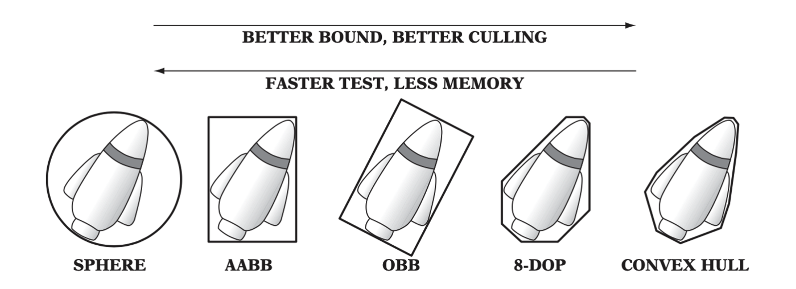
Types of bounding volumes: sphere, axis-aligned bounding box(AABB),oriented bounding box (OBB), eight-direction discrete orientation polytope (8-DOP), and convex hull.

Typesofboundingvolumes:sphere,axis-alignedboundingbox(AABB),oriented bounding box (OBB), eight-direction discrete orientation polytope (8-DOP), and convex hull.

Axis-aligned Bounding Boxes (AABBs)

The axis-aligned bounding box (AABB) is a rectangular six-sided box categorized by having its faces oriented in such a way that its face normals are at all times parallel with the axes of the given coordinate system.

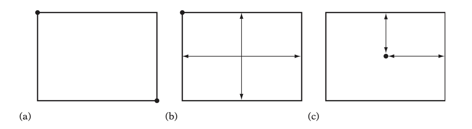
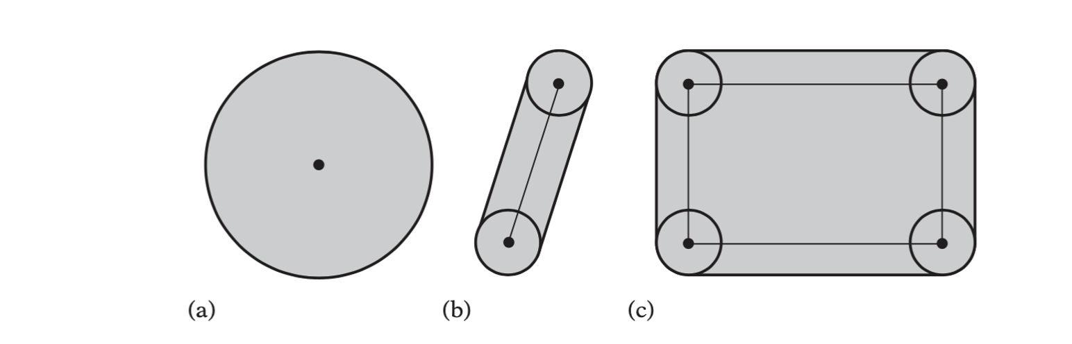
The three common AABB representations: (a) min-max, (b) min-widths, and (c) center-radius.

The three common AABB representations: (a) min-max, (b) min-widths, and (c) center-radius.

💡 In terms of storage requirements, the center-radius representation is the most efficient, as the halfwidth values can often be stored in fewer bits than the center position values.

AABB-AABB Intersection

Two AABBs only overlap if they overlap on all three axes.

int TestAABBAABB(AABB a, AABB b) {
	if (Abs(a.c[0] - b.c[0]) > (a.r[0] + b.r[0])) return 0;
	if (Abs(a.c[1] - b.c[1]) > (a.r[1] + b.r[1])) return 0;
	if (Abs(a.c[2] - b.c[2]) > (a.r[2] + b.r[2])) return 0;
	return 1;
}

Computing and Updating AABBs

Bounding volumes are usually specified in the local model space of the objects they bound(which may be world space).To perform an overlap query between two bounding volumes, the volumes must be transformed into a common coordinate system. The choice stands between transforming both bounding volumes into world space and transforming one bounding volume into the local space of the other.

For updating or reconstructing the AABB, there are four common strategies:

• Utilizing a fixed-size loose AABB that always encloses the object.
• Computing a tight dynamic reconstruction from the original point set.
• Computing a tight dynamic reconstruction using hill climbing.
• Computing an approximate dynamic reconstruction from the rotated AABB.

AABB from the Object Bounding Sphere

The fixed-size encompassing AABB is computed as the bounding box of the bounding sphere of the contained object. The benefit of this representation is that during update the AABB simply need be translated (by the same translation applied to the bounded object), and any object ortation can be completely ignored.

AABB Reconstructed from the Original Point Set

This strategy dynamically resizes the AABB as it is being realigned with the coordiante system axes. The straightforward approach loops through all vertices, keeping track of the vertex most distant along the direction vector. When \(n\) is large, the tight AABB can be constructed only by the vertices on the convex hull of the object.

When computing a tight AABB, only the highlighted vertices that lie on the convex hull of the object must be considered.

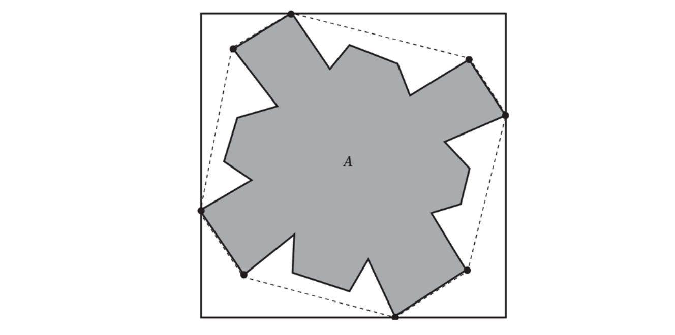
When computing a tight AABB, only the highlighted vertices that lie on the convex hull of the object must be considered.

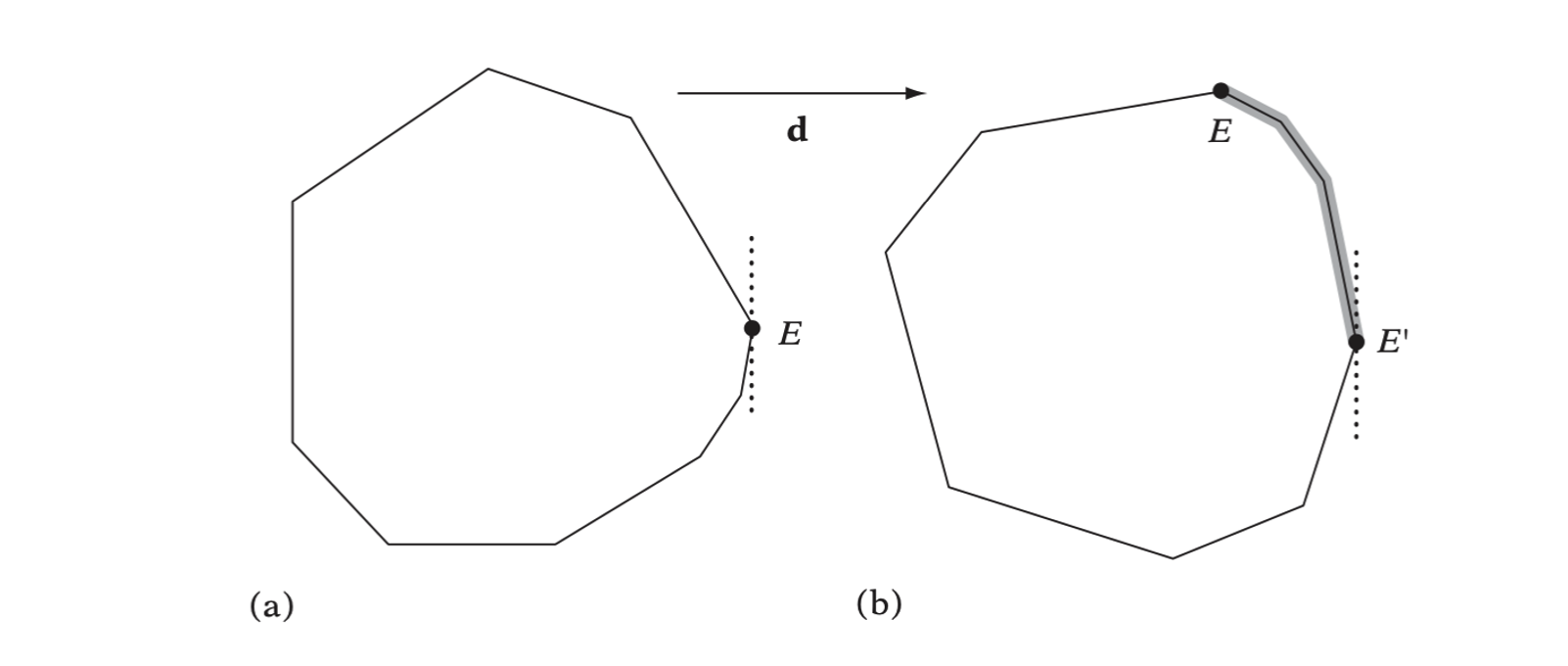
AABB from Hill-Climbing Vertices of the Object Representation

Instead of keeping track of the minimum and maximum extent values along each axis, six vertex pointers are maintained. Corresponding to the same values as before, these now actually point at the (up to six) extremal vertices of the object along each axis direction. The hill-climbing step now proceeds by comparing the referenced vertices against their neighbor vertices to see if they are still extremal in the same direction as before. Those that are not are replaced with one of their more extreme neighbors and the test is repeated until the extremal vertex in that direction is found. The hill-climbing process requires objects to be convex.

(a)The extreme vertex E in direction d. (b) After object rotates counterclockwise, the new extreme vertex E in direction d can be obtained by hill climbing along the vertex path highlighted in gray.

Spheres

Spheres are defined in terms of a center position and a radius:

struct Sphere {
	Point c; // Sphere center
	float r; // Sphere radius
}

Sphere-sphere Intersection

The Euclidean distance between the sphere centers is computed and compared against the sum of the sphere radii. To avoid an often expensive square root operation, the squared distances are compared.

int TestSphereSphere(Sphere a, Sphere b) {
	// Calculate the squared distance between centers.
	Vector d = a.c - b.c;
	float dist2 = Dot(d, d);
	// Spheres intersect if squared distance is less than squared sum of radii
	float radiusSum = a.r + b.r;
	return dist2 <= radiusSum * radiusSum; 
}

Computing a Bounding Sphere

The algorithm progresses in two passes.

• In the first pass
  • Six extremal points along the coordinate system axes are found.
  • Out of the six points, the pair of points farthest apart is selected.
  • The sphere center is now selected as the midpoint between these two points, and the radius is set to be half the distance between them.
• In the second pass
  • All points are looped throught again. For all points outside the current sphere, the sphere is updated to be the sphere just encompassing the old sphere and the outside point.

💡 By starting with a better approximation of the true bounding sphere, the resulting sphere could be expected to be even tighter.

Bounding Sphere from Direction of Maximum Spread

Instead of finding a pair of distant points using an AABB, a suggested approach is to analyze the point cloud using statistical methods to find its direction of maximum spread.

The same point cloud projected onto two different axes. In (a) the spread on the axis is small. In (b) the spread is much larger. A bounding sphere can be determined from the axis for which the projected point set has the maximum spread.

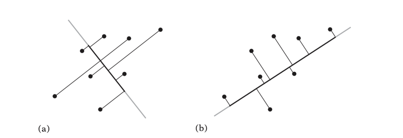
The same point cloud projected onto two different axes. In (a) the spread on the axis is small. In (b) the spread is much larger. A bounding sphere can be determined from the axis for which the projected point set has the maximum spread.

The mean is a measure of the central tendency of all values, variance is a messure of their dispersion. They are given by

\[ u = \frac{1}{n} \sum^n_{i=1} x_i \\ \sigma^2 = \frac{1}{n}\sum^n_{i = 1}(x_i - u)^2 = \frac{1}{n}\bigg(\sum^n_{i=1} x_i^2\bigg) - u^2 \]

For multiple variables, the covariance of the data is conventionally computed and expressed as a matrix, the covariance matrix. The covariance matrix \(\bold{C} = [c_{ij}]\) for a collection of \(n\) points \(P_1, P_2, \dots, P_n\) is given by

\[ c_{ij} = \frac{1}{n}\sum^n_{k = 1}(P_{k, i} - u_i)(P_{k, j} - u_j) \]

or equivalently by

\[ c_{ij} = \frac{1}{n}\bigg(\sum^n_{k=1}P_{k, i} P_{k, j}\bigg) - u_i u_j \]

where \(u_i\) is the mean of the \(i\)-th coordinate value of the points, given by

\[ u_i = \frac{1}{n}\sum^n_{k=1}P_{k, i} \]

The Minimum Bounding Sphere

Assume a minimum bounding sphere \(S\) has been computed for a point set \(P\). If a new point \(Q\) is added to \(P\), then only if \(Q\) lies outside \(S\) does \(S\) need to be recomputed. It is not difficult to see that \(Q\) must lie on the boundary of a new minimum bounding sphere for the point set \(P \cup \{ Q\}\).

Sphere WelzlSphere(
    Point pt[],
    unsigned int numPts,
    Point sos[],
    unsigned int numSos
) {
    // if no input points, the recursion has bottomed out. Now compute an
    // exact sphere based on points in set of support (zero through four points)
    if (numPts == 0) {
        switch (numSos) {
            case 0: return Sphere();
            case 1: return Sphere(sos[0]);
            case 2: return Sphere(sos[0], sos[1]);
            case 3: return Sphere(sos[0], sos[1], sos[2]);
            case 4: return Sphere(sos[0], sos[1], sos[2], sos[3]);
        }
    }
    // Pick a point at "random" (here just the last point of the input set)
    int index = numPts - 1;
    // Recursively compute the smallest bounding sphere of the remaining points
    Sphere smallestSphere = WelzlSphere(pt, numPts - 1, sos, numSos); // (*)
    // If the selected point lies inside this sphere, it is indeed the smallest
    if(PointInsideSphere(pt[index], smallestSphere))
        return smallestSphere;
    // Otherwise, update set of support to additionally contain the new point
    sos[numSos] = pt[index]
    // Recursively compute the smallest sphere of remaining points with new s.o.s.
    return WelzlSphere(pt, numPts - 1, sos, numSos + 1);
}

Oriented Bounding Boxes (OBBs)

An oriented bounding box (OBB) is a rectangular block, much like an AABB but with an arbitrary orientation. There are so many representations of OBB, following is one of them.

struct OBB {
    Point c; // OBB center point
    Vector u[3]; // Local x-, y-, and z-axes
    Vector e; // Positive halfwidth extends of OBB along each axis
}

OBB-OBB Intersection

Sphere-swept Volumes

(a) A sphere-swept point(SSP). (b) A sphere-swept line(SSL). (c) A sphere-swept rectangle (SSR).

Sphere-swept points (SSPs), sphere-swept lines (SSLs), and sphere-swept rectangles (SSRs) — are commonly referred to, respectively, as spheres, capsules, and lozenges.

struct Capsule {
    Point a; // Medial line segment start point
    Point b; // Medial line segment endpoint
    float r; // Radius
}
   
struct Lozenge {
    Point a; // Origin
    Vector u[2]; // The two edges axes of the rectangle
    float r; // Radius
};

Sphere-swept Volume Intersection

By construction, all sphere-swept volume tests can be formulated in the same way. First, the distance between the inner structures is computed. Then this distance is compared against the sum of the radii.

Halfspace Intersection Volumes

Although convex hulls form the tightest bounding volumes, they are not neces- sarily the best choice of bounding volume. Some drawbacks of convex hulls include their being expensive and difficult to compute, taking large amounts of memory to represent, and potentially being costly to operate upon. By limiting the number of halfspaces used in the intersection volume, several simpler alternative bounding volumes can be formed.

A slab is the infinite region of space between two planes, defined by a normal n and two signed distances from the origin.

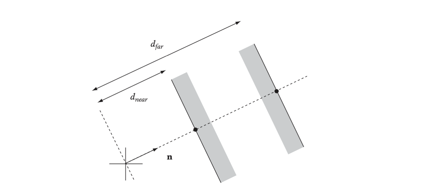
A slab is the infinite region of space between two planes, defined by a normal n and two signed distances from the origin.

struct Slab {
    float n[3]; // Normal n = (a, b, c)
    float dNear; // Signed distance from origin for near plane (dNear)
    float dFar; // Signed distance from origin for far plane (dFar)
};

To form a bounding volume, a number of normals are chosen. Then, for each normal, pairs of planes are positioned so that they bound the object on both its sides along the direction of the normal. To form a closed 3D volume, at least three slabs are required.

Discrete-orientation Polytopes (k-DOPs)

These k-DOPs are convex polytopes, almost identical to the slab-based volumes except that the normals are defined as a fixed set of axes shared among all k-DOP bounding volumes.

struct DOP8 {
    float min[4]; // Minimum distance (from origin) along axes 0 to 3
    float max[4]; // Maximum distance (from origin) along axes 0 to 3
}; 

An 8-DOP has faces aligned with the eight directions \((\pm1, \pm1, \pm1)\) and a 12-DOP with the 12 directions \((\pm1, \pm1, 0)\), \((\pm1, 0, \pm1)\) and \((0, \pm1, \pm1)\).

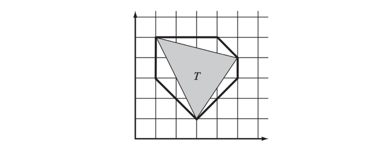
8-DOP for triangle (3,1),(5,4),(1,5) is {1,1,4,−4,5,5,9,2} for axes (1,0), (0,1), (1, 1), (1, −1).

8-DOP for triangle (3,1),(5,4),(1,5) is {1,1,4,−4,5,5,9,2} for axes (1,0), (0,1), (1, 1), (1, −1).

💡 Note that the k-DOP is not just any intersection of slabs, but the tightest slabs that form the body.

k-DOP-k-DOP Overlap Test

Due to the fixed set of axes being shared among all objects, the test simply checks the \(k/2\) intervals for overlap. If any pair of intervals do not overlap, the k-DOPs do not intersect.

int TestKDOPKDOP(KDOP &a, KDOP &b, int k) {
  // Check if any intervals are non-overlapping, return if so
  for (int i = 0; i < k / 2; i++)
    if (a.min[i] > b.max[i] || a.max[i] < b.min[i])
      return 0;

  // All intervals are overlapping, so k-DOPs must intersect
  return 1;
}

Computing and Realigning k-DOPs

Computing the k-DOP for an object can be seen as a generalization of the method for computing an AABB, much as the overlap test for two k-DOPs is really a generalization of the AABB-AABB overlap test. As such, a k-DOP is simply computed from the projection spread of the object vertices along the defining axes of the k-DOP.